www.hydrol-earth-syst-sci.net/16/4119/2012/ doi:10.5194/hess-16-4119-2012
© Author(s) 2012. CC Attribution 3.0 License.
Earth System
Sciences
Hydrologic system complexity and nonlinear dynamic concepts for a
catchment classification framework
B. Sivakumar1,2and V. P. Singh3
1School of Civil and Environmental Engineering, The University of New South Wales, Sydney, Australia 2Department of Land, Air and Water Resources, University of California, Davis, USA
3Department of Biological and Agricultural Engineering & Department of Civil and Environmental Engineering,
Texas A & M University, College Station, USA
Correspondence to: B. Sivakumar ([email protected])
Received: 12 April 2011 – Published in Hydrol. Earth Syst. Sci. Discuss.: 2 May 2011 Revised: 5 October 2012 – Accepted: 16 October 2012 – Published: 8 November 2012
Abstract. The absence of a generic modeling framework in
hydrology has long been recognized. With our current prac-tice of developing more and more complex models for spe-cific individual situations, there is an increasing emphasis and urgency on this issue. There have been some attempts to provide guidelines for a catchment classification frame-work, but research in this area is still in a state of infancy. To move forward on this classification framework, identi-fication of an appropriate basis and development of a suit-able methodology for its representation are vital. The present study argues that hydrologic system complexity is an ap-propriate basis for this classification framework and nonlin-ear dynamic concepts constitute a suitable methodology. The study employs a popular nonlinear dynamic method for iden-tification of the level of complexity of streamflow and for its classification. The correlation dimension method, which has its base on data reconstruction and nearest neighbor con-cepts, is applied to monthly streamflow time series from a large network of 117 gaging stations across 11 states in the western United States (US). The dimensionality of the time series forms the basis for identification of system complex-ity and, accordingly, streamflows are classified into four ma-jor categories: low-dimensional, medium-dimensional, high-dimensional, and unidentifiable. The dimension estimates show some “homogeneity” in flow complexity within certain regions of the western US, but there are also strong excep-tions.
1 Introduction
As in most other fields of science and engineering, growth in the field of hydrology during the past century has been unprecedented, largely driven by the invention of power-ful computers, measurement devices, remote sensors, geo-graphic information systems (GIS), digital elevation mod-els (DEM), and networking facilities. This growth may be viewed in terms of: (1) the various sub-fields that have been created essentially to “break down” hydrology into specific components for more focused and detailed studies (e.g. sur-face hydrology, subsursur-face hydrology, groundwater hydrol-ogy, forest hydrolhydrol-ogy, mountain hydrolhydrol-ogy, urban hydrolhydrol-ogy, isotope hydrology, snow and glacier hydrology, ecohydrol-ogy); and (2) the numerous scientific theories and mathemat-ical techniques that have been developed/applied for model-ing and prediction of hydrologic systems and the associated processes (e.g. deterministic techniques, stochastic methods, scaling and fractal theories, artificial neural networks, chaos theory, wavelets, entropy theory, evolutionary computing).
between the (model) theories and the actual system proper-ties (e.g. data), our increasing emphasis in applying specific (and often pre-selected) mathematical techniques indepen-dently as opposed to the integration of techniques for model-ing hydrologic systems, and our focus mainly on local-scale hydrologic problems rather than global-scale hydrologic is-sues have also come under severe scrutiny (e.g. Beven, 2002; Sivakumar, 2008). With growing concerns on the occurrence of global climate change and its potential impacts on wa-ter resources and the environment (including more frequent and greater magnitudes of extreme events, such as floods and droughts), the limitations of the “confines of traditional hydrology” and the need to go beyond and perform cross-disciplinary research integrating hydrology with atmospheric science, geomorphology, geochemistry, ecology, and other areas have also been increasingly recognized (see, for exam-ple, Paola et al., 2006, for some details).
In view of these concerns, many studies during the past decade or so have emphasized the need for simplification in modeling wherever possible as well as a common framework in hydrology (e.g. Grayson and Bl¨oschl, 2000; McDonnell and Woods, 2004). Within this context, some attempts have also been made towards a catchment classification frame-work (e.g. Snelder et al., 2005; Sivakumar et al., 2007; see also the other articles in the current special issue “Catch-ment Classification and PUB” for some latest studies), with an aim to streamline catchments into different groups and sub-groups on the basis of their salient characteristics (e.g. data and process complexity) and to provide directions to model developers on the level of model complexity to in-voke. Nevertheless, these attempts are only preliminary and research in this direction is still in a state of infancy. Indeed, there are even questions on the basic form of the classifica-tion framework and on the components to be included (e.g. Wagener et al., 2007). Therefore, identification of an appro-priate basis for the classification framework and development of a suitable methodology are crucial for moving forward in hydrology.
The present study attempts to offer some workable guide-lines for an appropriate basis and a suitable methodology to-wards a classification framework in hydrology. The study ar-gues, through highlighting the relevance of complexity and nonlinearity in hydrologic systems, that system complexity is an appropriate basis for the classification framework and nonlinear dynamic concepts constitute a suitable methodol-ogy for assessing system complexity. With this, it examines the usefulness of a nonlinear dynamic method for stream-flow classification. This is done by employing the corre-lation dimension method (e.g. Grassberger and Procaccia, 1983a) to streamflow from a large network of gaging stations in the western United States. Monthly streamflow data ob-served over a period of 52 yr from 117 gaging stations across 11 states are considered for analysis. The identification of the level of complexity and the subsequent classification are
made based on the dimensionality of the streamflow time se-ries.
The rest of this paper is organized as follows. Section 2 presents a brief account of major attempts on classification in hydrology. Section 3 highlights the role of complexity and nonlinearity in hydrologic systems. Section 4 describes the correlation dimension method. Section 5 presents the details of streamflow data from the western United States and re-sults of their analysis. Conclusions and directions for further research are presented in Sect. 6.
2 Classification in hydrology: a brief history and scope
The realization of the need for a classification framework in hydrology is not entirely new. It had indeed been dis-cussed some time ago, and since then several studies have also attempted to advance the idea. These studies have inves-tigated different ways for developing such a framework and their implications, including river morphology (e.g. Rosgen, 1994; Poff et al., 2006), river/flow regimes (e.g. Beckinsale, 1969; Haines et al., 1988), landscape and land use parameters (e.g. Merz and Bl¨oschl, 2004; Wardrop et al., 2005), simi-larity indices (e.g. Olden and Poff, 2003; Ali et al., 2012), eco-hydrologic factors (e.g. Harris et al., 2000; Olden et al., 2011), geostatistical properties (e.g. Vormoor et al., 2011), entropy (e.g. Krasovkaia, 1997), nonlinear and chaotic dy-namic properties (e.g. Sivakumar et al., 2007), and other rel-evant characteristics/methods (e.g. Chapman, 1989; Isik and Singh, 2008). Extensive details of these studies are available both in the traditional hydrologic literature and in related fields (e.g. geomorphology, ecohydrology, and freshwater bi-ology); for some very latest accounts, see Ali et al. (2012) and also the articles in the current special issue “Catchment Classification and PUB.”
Although useful in their own ways, these studies are largely inadequate for a generic classification framework. In addition to the limitations that exist in each of the different forms, a coherent effort to bring these disparate forms to-gether for a workable classification framework is also miss-ing. The urgency to formulate a generic classification frame-work in hydrology is increasingly realized now, especially with our current practice of employing more and more so-phisticated mathematical techniques and developing more and more complex models for each and every individual hy-drologic system/situation, rather than the emphasis needed for addressing broader-scale hydrologic issues (e.g. Sivaku-mar, 2008).
(2) treatment of each and every individual hydrologic system in its own way, regardless of the similarities among them. Ei-ther of these approaches has enormous implications for mod-eling, including complexity of the models, data and computer requirement, accuracy of results, and overall understanding of the systems. The classification framework, therefore, is aimed at providing an optimum way of studying hydrologic systems, taking into account both minimization of costs and maximization of benefits. In the end, it should help modelers identify suitable catchments to apply their models to and also users to identify suitable models for their catchments.
For its usefulness to be realized both at the global and at the regional/local levels, the classification framework should be able to accommodate important general as well as specific characteristics of hydrologic systems/processes. The frame-work must also be simple enough and commonly agree-able to provide a “universal” language for communication and discussion in hydrology and water resources. The cru-cial questions now are: (1) What form should the classifi-cation framework assume? (2) What components need to be included? (3) What is the appropriate methodology for its formulation? and (4) How to effectively verify such a classi-fication framework? A few studies have attempted to address these questions and relevant issues, such as the examples be-low.
Wagener et al. (2007) reviewed the existing approaches to define hydrologic similarity, which has often been in-voked for classification purposes, and offered some gen-eral guidelines for catchment classification that include the use of catchment structure, hydro-climatic region, and catch-ment functional response, among others. They also identified the following requirements for a classification framework: (1) mapping catchment form/hydro-climatic conditions on catchment function across spatial and temporal scales; (2) in-cluding partition, storage, and release of water in catch-ment functions; (3) consideration of uncertainty in the met-rics/variables used; and (4) basing on functions characterized by streamflow to start with and subsequently expanding to other more complex functions.
Using the Shannon entropy, Krasovskaia (1995, 1997) de-veloped a quantitative methodology for studying river flow regimes and their classification. The entropy-based method-ology involves: (1) classification of mean monthly flows into different types; (2) identification of discriminating periods for different classes; (3) specification of instability index; (4) computation of instability index value for each regime type; and (5) computation of instability index for all flow se-ries. Another method for grouping river regimes, developed by Krasovskaia (1997), employs minimization of an entropy-based objective function. This function uses a concept of information loss resulting from flow aggregation and deter-mining the difference between the series aggregated into one group.
Sivakumar et al. (2007) explored the utility of a simple nonlinear data reconstruction approach, called phase space
reconstruction, for assessing the complexity of hydrologic systems and, thus, for their classification. They used the “re-gion of attraction of trajectories” in the phase space to iden-tify data as exhibiting “simple” or “intermediate” or “com-plex” behavior and, correspondingly, classify the system as potentially low-, medium-, or high-dimensional. The utility of this reconstruction concept was first demonstrated on two artificial time series possessing significantly different char-acteristics and levels of complexity (purely random and low-dimensional deterministic), and then tested on a host of river-related data representing different geographic regions, cli-matic conditions, basin sizes, processes, and scales. The abil-ity of the phase space to reflect the river basin characteristics and the associated mechanisms, such as basin size, smooth-ing, and scalsmooth-ing, was also observed. The “dimensionality” and “complexity” ideas used by Sivakumar et al. (2007) were along the lines of the dominant processes concept (DPC), which was originally introduced in the context of hydrologic model simplification (Grayson and Bl¨oschl, 2000) and sub-sequently suggested as a potential means for formulation of a classification framework (e.g. Woods, 2002; Sivakumar, 2004a).
Following up on the preliminary ideas by Sivakumar et al. (2007) based on just a few example cases, we attempt here to advance the studies on nonlinear dynamic concepts for identifying complexity of hydrologic systems and for their classification. To this end, we particularly consider that the extent of “complexity” of the system is reflected by the “vari-ability” of the representative (observed) data (i.e. streamflow in the present case), which, in turn, is assessed by its “di-mensionality”. We apply the correlation dimension method for studying data dimensionality and system complexity, and use such information for classification purposes.
3 Complexity and nonlinearity in hydrologic systems
3.1 Complexity in hydrologic systems
to identify the complexity of one system and to compare it with the complexity of another system? To develop a quanti-tative understanding of complexity, a variety of tools can be used. These may include: statistical (e.g. coefficient of varia-tion), nonlinear dynamic (e.g. dimension), information theo-retic (e.g. entropy), or some other measure. In this study, we discuss the nonlinear dynamic tools, which allow identifica-tion of complexity of different systems and interpretaidentifica-tions and distinctions on “more complex” and “less complex” sys-tems. In particular, we attempt to assess the complexity of the system in terms of variability of the data through dimension estimation.
Hydrologic phenomena arise as a result of interactions be-tween climate inputs and landscape characteristics that oc-cur over a wide range of space and time scales. Due to the tremendous heterogeneities in climatic inputs and land-scape properties, such phenomena may be highly variable and “complex” at all scales. Consequently, they are not fully understood. In the absence of perfect knowledge, a simpli-fied way to represent them may be through the concept of “system”. There are many different definitions of a system, but perhaps the simplest may be: “a system is a set of con-nected parts that form a whole”. Chow (1964) defined a sys-tem as an aggregate or assemblage of parts, being either ob-jects or concepts, united by some form of regular interaction or inter-dependence. Dooge (1967a), however, defined a sys-tem as: “any structure, device, scheme, or procedure, real or abstract, that inter-relates in a given time reference, an input, cause, or stimulus, of matter, energy, or information and an output, effect, or response of information, energy, or matter”. This definition by Dooge is much more comprehensive and instructive.
With this system concept, the entire hydrologic cycle may be regarded as a hydrologic system, whose components might include precipitation, interception, evaporation, tran-spiration, infiltration, detention storage or retention storage, surface runoff, interflow, and groundwater flow, and perhaps other phases of the hydrologic cycle. Each component may be treated as a sub-system of the overall cycle, if it satisfies the characteristics of a system set out in its definition. Thus, the various components of the hydrologic system can be re-garded as hydrologic sub-systems. To analyze the total sys-tem, the simpler sub-systems can be treated separately and the results combined according to the interactions between the sub-systems (especially with the assumption of linear-ity). Whether a particular component is to be treated as a system or sub-system depends on the “objective of the in-quiry” (Singh, 1988).
In this “objective of the inquiry” context, Sivaku-mar (2008) suggests that hydrologic systems may be viewed from three different, but related, angles: process, scale, and purpose of interest. Depending upon the angle at which they are viewed, hydrologic systems may be either simple or com-plex; for example, the rainfall occurrence in a desert may be treated as an extremely simple process since there may be
no rainfall at all, while the runoff process in a large river basin may be highly complex due to the basin complexities and heterogeneities, in addition to rainfall variability. Conse-quently, hydrologic modeling must also be viewed from these three angles; in other words, the appropriate model to repre-sent a given hydrologic system may also be either simple or complex. The obvious question, however, is: how simple or how complex should the models be? This issue is addressed in this study, since the basic purpose behind formulation of a catchment classification framework is the identification of the most appropriate model (type and complexity) for a given catchment.
Since complexity is a fundamental and central characteris-tic of hydrologic systems, and is also a representation of their generality and specificity, it should form the basis for a clas-sification framework. The study by Sivakumar et al. (2007), for example, offers some clues as to the use of complexity (defined in terms of extent of data variability) as a viable means for a classification framework.
3.2 Nonlinearity in hydrologic systems
Much of the research in hydrologic systems, at least until the 1990s, has been based on the assumption of “linearity”; i.e., the relation between cause (e.g. input) and effect (e.g. output) is linear or proportional. One of the important fac-tors that contributed to, or necessitated, this linear approach was the lack of computational power to develop the (perhaps more complex) nonlinear mathematical methods. However, the “nonlinear” behavior of hydrologic systems had been known for a long time (e.g. Izzard, 1966; Dooge, 1967b).
The nonlinear behavior of hydrologic systems is evident in various ways and at almost all spatial and temporal scales. The hydrologic cycle itself is an example of a system ex-hibiting nonlinear behavior, with almost all of the individ-ual components themselves exhibiting nonlinear behavior as well. The climatic inputs and landscape characteristics are changing in a highly nonlinear fashion, and so are the out-puts, often in unknown ways. The rainfall-runoff process is nonlinear, almost regardless of the basin area, land uses, rain-fall intensity, and other influencing factors. In fact, the ef-fects of nonlinearity can be tremendous, especially when the system is sensitively dependent on initial conditions. This means, even small changes in the inputs may result in large changes in the outputs (and large changes in the inputs may turn out to cause only small changes in the outputs), a sit-uation popularly termed as “chaos” in the nonlinear science literature (e.g. Lorenz, 1963).
models (e.g. Young and Beven, 1994), and nonlinear dynam-ics and chaos (e.g. Sivakumar, 2000) are some of the popular nonlinear techniques that have found extensive applications in hydrology. This study discusses the utility of nonlinear dy-namic techniques as a suitable methodology for studying the complexity of hydrologic systems and, thus, for formulation of a catchment classification framework. In particular, we ap-ply a popular nonlinear dynamic method, the correlation di-mension method, to streamflow time series for classification purposes.
4 Correlation dimension method
During the past three decades or so, significant advances have been made in the field of nonlinear sciences to study complex systems. Numerous methods have been developed and ap-plied in various fields, including physics, chemistry, biology, earth sciences, ecology, economics, engineering, medicine, and psychology. Extensive details of the applications of non-linear dynamics and chaos concepts in hydrology are found in Sivakumar (2000) and in the broader field of geophysics in Sivakumar (2004b).
Popular among the methods developed within the con-text of nonlinear dynamic and chaos theories are correla-tion dimension, Lyapunov exponent, false nearest neighbors, nonlinear prediction, surrogate data, and redundancy meth-ods. Almost all of these methods involve data embedding and nearest neighbor search, identifying different yet related properties of the underlying system dynamics. In this study, we employ the correlation dimension method for complexity determination of time series.
Correlation dimension is a measure of the extent to which the presence of a data point affects the position of the other points lying on the attractor in (a multi-dimensional) phase space or coordinate system. The correlation dimension method uses the correlation integral (or function) for deter-mining the dimension of the attractor in the phase space and, hence, for distinguishing, broadly, between low-dimensional and high-dimensional systems. The concept of the correla-tion integral is that a time series arising from deterministic dynamics will have a limited number of degrees of freedom equal to the smallest number of first-order differential equa-tions that capture the most important features of the dynam-ics. Thus, when one constructs phase spaces of increasing di-mension, a point will be reached where the dimension equals the number of degrees of freedom, beyond which increasing the phase space dimension will not have any significant effect on correlation dimension.
Many algorithms have been formulated for the estima-tion of the correlaestima-tion dimension of a time series. Among these, the Grassberger–Procaccia algorithm (Grassberger and Procaccia, 1983a) has been and continues to be the most widely used one, especially in hydrologic studies. The al-gorithm uses the concept of phase space reconstruction (e.g.
Packard et al., 1980) for representing the dynamics of the system from an available single-variable time series. Given a single-variable series,Xi, where i=1, 2, ...,N, a multi-dimensional phase space can be reconstructed as (Takens, 1981):
Yj=(Xj, Xj+τ, Xj+2τ, ..., Xj+(m−1)τ), (1)
wherej =1, 2, ...,N−(m−1)τ;mis the dimension of the vectorYj, called embedding dimension; andτ is an
appro-priate delay time, which is an integer multiple of sampling time. It must be noted that if time series of multiple variables are available (e.g. relevant climate and hydrologic variables influencing streamflow dynamics, such as rainfall, tempera-ture, and infiltration), then such can be directly used for re-construction, which will be a more realistic representation of the system dynamics and, thus, will yield more reliable re-sults.
A correct phase space reconstruction in a dimension m
generally allows interpretation of the system dynamics (if the variable chosen to represent the system is appropriate) in the form of an m-dimensional mapfT, given by
Yj+T =fT(Yj), (2)
whereYj andYj+T are vectors of dimensionm, describing
the state of the system at timesj (current state) and j+T
(future state), respectively.
For an m-dimensional phase space, the correlation func-tionC(r)is given by
C(r)= lim
N→∞
2
N (N−1)
X
i,j
H r−Yi−Yj
, (3)
(i≤i<j≤N )
whereH is the Heaviside step function, withH (u)=1 for
u >0, andH (u)=0 foru≤0, whereu=r− kYi−Yjk,r
is the vector norm (radius of sphere) centered onYi orYj. If
the time series is characterized by an attractor, thenC(r)and
rare related according to
C(r)≈αrν,
r→0
N→ ∞
(4)
whereαis a constant andνis the correlation exponent or the slope of the LogC(r)versus Logrplot. The slope is gener-ally estimated by a least square fit of a straight line over a certain range ofr(i.e. scaling regime) or through estimation of local slopes between r-values.
of the number of variables dominantly governing the sys-tem dynamics. Although the correlation dimension method is widely used for distinguishing low-dimensional systems and high-dimensional systems, additional categories of system dimensionality (e.g. medium) can also be formed based on correlation dimension values. This is attempted in the present study to achieve better grouping of streamflow time series.
It is relevant to note, at this point, that the reliability of the Grassberger–Procaccia algorithm (or any other algorithm for that matter) for correlation dimension estimation of real time series (e.g. streamflow observations) has been under consid-erable debate, in view of the potential limitations that may exist with the method and/or the data. Some of the relevant is-sues are data size (e.g. Havstad and Ehlers, 1989), data noise (e.g. Schreiber and Kantz, 1996), presence of zeros (e.g. Tso-nis et al., 1994), temporal correlations and delay time selec-tion for phase space reconstrucselec-tion (e.g. Fraser and Swinney, 1986), even stochastic processes yielding low correlation di-mensions (e.g. Osborne and Provenzale, 1989), and others. As most of these issues are also highly relevant to hydrologic time series, there have been criticisms on the correlation di-mension estimates reported for hydrologic time series as well (e.g. Schertzer et al., 2002; Koutsoyiannis, 2006).
Numerous studies have addressed these issues and allayed the concerns on the reliability of correlation dimension esti-mates of hydrologic time series. Indeed, some studies have pointed out that many of the criticisms on dimension esti-mates are often unreliable and unfounded; see Sivakumar et al. (2002a) in response to Schertzer et al. (2002) regard-ing the issue of data size. These issues and concerns as well as clarifications and interpretations regarding correlation di-mension estimates of hydrologic time series have already been extensively discussed in the literature (e.g. Sivakumar, 2000; Sivakumar et al., 2002b). Therefore, further details are not reported herein, and the interested reader is directed to such studies. However, as the issue of data size is particularly relevant for the 117 streamflow time series analyzed in this study (with “only” 624 values in each series), we will briefly discuss the reliability of our correlation dimension estimates in Sect. 5.3. We will also briefly explain our selection of the delay time for phase space reconstruction and its implica-tions.
5 Data, analysis, and results
5.1 Data
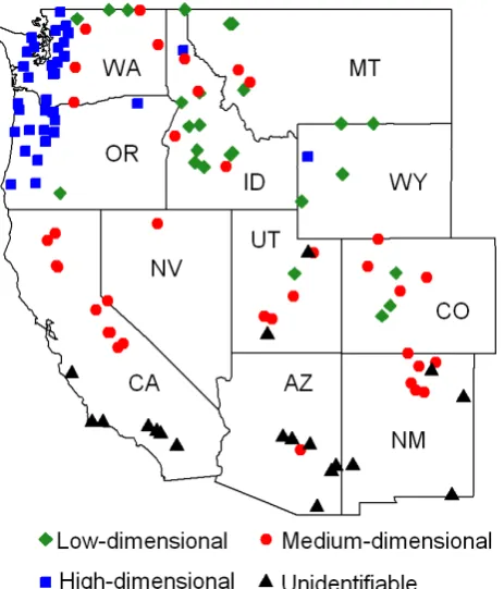
[image:6.595.312.546.63.257.2]In this study, monthly streamflows from the western United States (US) are studied, with data collected over an exten-sive network of 117 gaging stations (see Fig. 1). The sta-tions are spread over 11 states in the western US: Arizona (AZ), California (CA), Colorado (CO), Idaho (ID), Mon-tana (MT), Nevada (NV), New Mexico (NM), Oregon (OR), Utah (UT), Washington (WA), and Wyoming (WY). The
Fig. 1. Map of the western United States and locations of 117 streamflow gaging stations. AZ – Arizona; CA – California; CO – Colorado; ID – Idaho; MT – Montana; NM – New Mexico; NV – Nevada; OR – Oregon; UT – Utah; WA – Washington; WY – Wyoming.
drainage areas range from as small as 22.79 km2 (8.8 mi2)
(Station #11058500 in California) to as large as 35 094 km2 (13 550 mi2)(Station #13317000 in Idaho); as many as two-thirds of the catchments are small- to medium-sized, i.e. less than 1000 km2(or approximately 400 mi2).
Streamflow data in the US are commonly expressed in “water years”, which commence in October. The records used in this study are those observed over a period of 52 yr, starting in October 1951 and ending in September 2003, and are average monthly streamflow values. The magnitude of streamflow varies greatly among the 117 stations (e.g. even during the same period) as well as within a station (e.g. at dif-ferent periods). Notable observations of the flow variations (during the 52-yr period of 1951–2002) are as follows:
– the mean flows range from as low as 0.06 m3s−1
(1.97 ft3s−1) at Station #11063500 in CA to as high as
322 m3s−1(11 550 ft3s−1) at Station #13317000 in ID;
– the standard deviation values range from as low as
0.11 m3s−1 (3.92 ft3s−1) at Station #11063500 to as high as 373.5 m3s−1 (13 193 ft3s−1) at Station #13317000;
– the coefficient of variation (CV) values (defined as the
standard deviation divided by the mean) range from as low as 0.295 at Station #11367500 in CA to to as high as 4.324 at Station #10258500 in CA;
– the maximum flow observed was 2339 m3s−1
– flows over 300 m3s−1(or about 10 000 ft3s−1) were
ob-served at 18 stations and flows less than 0.3 m3s−1(or
about 10 ft3s−1) were observed at 38 stations (23
sta-tions if those having zero flows are excluded); and
– five stations (Station #9448500, #9498500, #9508500,
#12401500, and #14301000) had a maximum flow of over 300 m3s−1(about 10 000 ft3s−1) and also a mini-mum flow of less than 3 m3s−1(about 100 ft3s−1). All these observations clearly reflect the extreme variabil-ity in streamflow among the 117 stations. The variabilvariabil-ity in streamflow is due to, among others: (1) the different cli-matic regions in the western US; (2) the different drainage basin characteristics associated with the streamflow stations; and (3) the variations in hydroclimatic factors and land-use changes over a period of time at any of these stations.
Further details on these 117 streamflow stations in the western US (as well as the numerous other ones in the conterminous US), including streamflow data retrieval, are available at: http://nwis.waterdata.usgs.gov/nwis. The reader is also directed to Sivakumar (2003) and Tootle and Piechota (2006) for some of the studies relevant to stream-flow at these stations.
5.2 Analysis and results
The correlation dimension analysis is performed on each of the above 117 streamflow time series. The phase space di-agrams and the correlation exponent plots (i.e. local slope versus logr) are carefully interpreted to achieve appropriate grouping of these time series.
Both phase space diagrams and correlation dimension plots show varying degrees of results among the 117 time series. The phase space diagrams exhibit attractors ranging from reasonably well-structured ones (i.e. in a well-defined region in the phase space) to totally “shapeless” ones (i.e. dif-ficult to identify any kind of structure), and others in between these two extremes. Similarly, the correlation exponent plots show dimensionalities ranging from very low values of satu-ration ofνat one extreme (say less than 3) to unidentifiable ones at the other, and others in between.
Based on careful examination of phase space diagrams and correlation dimension results of all 117 streamflow se-ries, we are able to identify four reasonably distinct groups. This identification is made based on the dimensionality of the attractor (d, i.e. saturation value of ν) as the primary criterion, since the dimensionality results allow a slightly better interpretation (qualitatively and quantitatively) com-pared to phase space diagrams. However, we also place par-ticular emphasis on the consistency between dimensionality and attractor shape (phase space diagram) for each group, for a more reliable grouping. The four groups and the asso-ciated dimensionalities are as follows: (1) low-dimensional, withd≤3.0; (2) medium-dimensional, with 3.0< d≤6.0; (3) high-dimensional, with d >6.0; and (4) unidentifiable.
The selection of the number of groups and the range of di-mension values for each group is somewhat arbitrary. Never-theless, they are certainly reasonable, especially in the con-text of the number of stations studied in the present study, since too many groups (with only minor differences among them) or just two groups (e.g. high-dimensional and low-dimensional) do not really serve the purpose of classification of 117 time series. Further, the above grouping according to correlation dimensions is also reasonable in the context of process/model complexity, since the influence of more than six dominant governing variables (i.e.d >6.0) often leads to high complexity in dynamics (requiring “complex” models), whereas that of 3 or less variables can confidently be consid-ered to lead to simpler dynamics (requiring “simple” mod-els), with other in between (medium-complexity dynamics, requiring medium-complexity models).
For discussion here, we present the results for two time series from each of these four groups. The stations repre-senting these time series are as follows: (1) low-dimensional – Station #10032000 (WY) and Station #13317000 (ID); (2) medium-dimensional – Station #11315000 (CA) and Station #11381500 (CA); (3) high-dimensional – Sta-tion #12093500 (WA) and StaSta-tion #14185000 (OR); and (4) unidentifiable – Station #8408500 (NM) and Station #11124500 (CA).
Figure 2a–h presents the phase space diagrams for stream-flow series from the above eight stations. The diagrams corre-spond to the reconstruction in two dimensions (m=2) with delay time τ=1, i.e. the projection of the attractor on the plane {Xi, Xi+1}. The following general observations may
be made: (1) the plots on the first row exhibit reasonably well-structured attractors in the phase space, suggesting that the systems are likely less complex and low-dimensional; (2) the second row plots indicate slightly wider scattering of the attractor, suggesting systems of medium complexity and medium dimension; (3) the plots on the third row exhibit much wider scattering (especially with one or a few outliers), suggesting highly complex and high-dimensional systems; and (4) the last two plots do not show any identifiable pat-terns, thus making it hard to include them in any of the above three groups.
Figure 3a–h presents the correlation dimension results for the above eight streamflow series; the plots show the local slopes (i.e. correlation exponent,ν)as a function of radius,
(a) (b) (c) (d) 0 10 20 30 40 50
0 10 20 30 40 50
Flo
w
(m
3s -1), X
i+1
Flow (m3s-1), Xi
0 500 1000 1500 2000 2500
0 500 1000 1500 2000 2500
Flo
w
(m
3s -1), X
i+1
Flow (m3s-1), Xi
0 4 8 12 16 20
0 4 8 12 16 20
Flo
w
(m
3s -1), X
i+1
Flow (m3s-1), Xi
0 10 20 30 40 50 60
0 10 20 30 40 50 60
Flo
w
(m
3s -1), X
i+1
Flow (m3s-1), X i (a) (b) (c) (d) 0 10 20 30 40 50
0 10 20 30 40 50
Flo
w
(m
3s -1), X
i+1
Flow (m3s-1), Xi
0 500 1000 1500 2000 2500
0 500 1000 1500 2000 2500
Flo
w
(m
3s -1), X
i+1
Flow (m3s-1), Xi
0 4 8 12 16 20
0 4 8 12 16 20
Flo
w
(m
3s -1), X
i+1
Flow (m3s-1), Xi
0 10 20 30 40 50 60
0 10 20 30 40 50 60
Flo
w
(m
3s -1), X
i+1
Flow (m3s-1), Xi
(e) (f) (g) (h) 0 15 30 45 60 75 90
0 15 30 45 60 75 90
Flo
w
(m
3s -1), X
i+1
Flow (m3s-1), X i 0 30 60 90 120 150
0 30 60 90 120 150
Flo
w
(m
3s -1), X
i+1
Flow (m3s-1), Xi
0 5 10 15 20 25
0 5 10 15 20 25
Flo
w
(m
3s -1), X
i+1
Flow (m3s-1), X i 0 5 10 15 20 25
0 5 10 15 20 25
Flo
w
(m
3s -1), X
i+1
Flow (m3s-1), Xi
(e) (f) (g) (h) 0 15 30 45 60 75 90
0 15 30 45 60 75 90
Flo
w
(m
3s -1), X
i+1
Flow (m3s-1), X i 0 30 60 90 120 150
0 30 60 90 120 150
Flo
w
(m
3s -1), X
i+1
Flow (m3s-1), X i 0 5 10 15 20 25
0 5 10 15 20 25
Flo
w
(m
3s -1), X
i+1
Flow (m3s-1), X i 0 5 10 15 20 25
0 5 10 15 20 25
Flo
w
(m
3s -1), X
i+1
[image:8.595.49.284.64.398.2]Flow (m3s-1), X i
Fig. 2. Phase space diagram: (a) Station #10032000; (b) Station #13317000; (c) Station #11315000; (d) Station #11381500; (e) Sta-tion #12093500; (f) StaSta-tion #14185000; (g) StaSta-tion #8408500; and (h) Station #11124500.
highly complex systems; and (4) the results for the last two series do not show any clear indication regarding the dimen-sion value or group (as they show neither saturation ofνnor high-dimensionality) and, therefore, are considered “uniden-tifiable”.
At this point, a few remarks about the identification of the scaling region and estimation of the correlation exponent are in order. As mentioned earlier, the scaling region can be iden-tified in the following ways: (1) identifying the long “straight line” portion in the LogC(r)versus Logrplot (i.e. correla-tion funccorrela-tion versus radius); and (2) the “horizontal line” in the local slope versus Logrplot. It is important to note that a “perfect straight line” or a “perfect horizontal line” in these plots may be found when the data are completely clean, but is often very hard to find when the data are noisy, as is the case with streamflow (and other hydrologic) data; the higher the embedding dimension (or attractor dimension), the harder it is to find the scaling region. Also, when the data are noisy, the slopes are hard to find at small r-values, and there is normally a shift in the r-values that yield the best results;
(a) (b) (c) (d) 0 1 2 3 4 5 6
3.3 3.7 4.1 4.5 4.9 5.3
Lo ca l S lo p e Log r 0 1 2 3 4 5 6
1.0 1.3 1.6 1.9 2.2 2.5 2.8 3.1
Lo ca l S lo p e Log r 0 1 2 3 4 5 6
1.4 1.8 2.2 2.6 3.0 3.4 3.8
Lo ca l S lo p e Log r 0 2 4 6 8
1.6 2.0 2.4 2.8 3.2 3.6
Lo ca l S lo p e Log r (a) (b) (c) (d) 0 1 2 3 4 5 6
3.3 3.7 4.1 4.5 4.9 5.3
Lo ca l S lo p e Log r 0 1 2 3 4 5 6
1.0 1.3 1.6 1.9 2.2 2.5 2.8 3.1
Lo ca l S lo p e Log r 0 1 2 3 4 5 6
1.4 1.8 2.2 2.6 3.0 3.4 3.8
Lo ca l S lo p e Log r 0 2 4 6 8
1.6 2.0 2.4 2.8 3.2 3.6
Lo ca l S lo p e Log r (e) (f) (g) (h) 0 2 4 6 8 10 12
1.4 1.8 2.2 2.6 3.0 3.4 3.8
Lo ca l S lop e Log r 0 1 2 3 4 5 6
0.8 1.2 1.6 2.0 2.4 2.8 3.2
Lo ca l S lo p e Log r 0 2 4 6 8 10 12
1.6 2.0 2.4 2.8 3.2 3.6 4.0
Lo ca l S lo p e Log r 0 1 2 3 4 5 6
0.8 1.2 1.6 2.0 2.4 2.8 3.2
Lo ca l S lo p e Log r (e) (f) (g) (h) 0 2 4 6 8 10 12
1.4 1.8 2.2 2.6 3.0 3.4 3.8
Lo ca l S lop e Log r 0 1 2 3 4 5 6
0.8 1.2 1.6 2.0 2.4 2.8 3.2
Lo ca l S lo p e Log r 0 2 4 6 8 10 12
1.6 2.0 2.4 2.8 3.2 3.6 4.0
Lo ca l S lo p e Log r 0 1 2 3 4 5 6
0.8 1.2 1.6 2.0 2.4 2.8 3.2
Lo ca l S lo p e Log r
Fig. 3. Correlation dimension – Local slopes: (a) Station #10032000; (b) Station #13317000; (c) Station #11315000; (d) Sta-tion #11381500; (e) StaSta-tion #12093500; (f) StaSta-tion #14185000; (g) Station #8408500; and (h) Station #11124500.
again, the difficulty increases at higher embedding dimen-sions (and higher attractor dimendimen-sions). Therefore, it is often helpful, and necessary, to use as many ways as possible to be more confident of the scaling region identification and cor-relation exponent estimation. Further details on the effects of noise on the correlation dimension estimate, in particular reference to hydrologic data (rainfall), are presented in, for example, Sivakumar et al. (1999b), and the interested reader is directed to such.
[image:8.595.312.546.64.408.2]
Fig. 4. Grouping of streamflow stations according to
cor-relation dimension (d) estimates: low-dimensional (d≤3.0);
medium-dimensional (3.0< d≤6.0); high-dimensional (d >6.0);
and unidentifiable (dnot identifiable).
Figure 4 presents the grouping of the 117 streamflow time series in the western US, according to the above dimension-ality (and phase space) criterion. The grouping show some kind of “homogeneity” in the dimensionality and complexity of streamflow dynamics within certain regions. For instance: (1) streamflow dynamics in the far northwest (i.e. west-ern parts of WA and OR) are generally high-dimensional; (2) the dimensionality of streamflows in the far south and southwest (southern CA, southern AZ, southern NM) is generally unidentifiable; (3) the complexity of streamflow dynamics in the west (northern CA and NV) is generally medium-dimensional; and (4) low-dimensional complexity is generally observed for streamflows in Wyoming. However, this “homogeneity” is not true for every region, and there are indeed strong exceptions. For example: (1) both low-dimensional and medium-low-dimensional complexity of stream-flow dynamics are observed in some other regions, especially in the east and north (including CO, ID, MT, and some parts of WA); and (2) streamflow dynamic complexity in some re-gions is rather very mixed, ranging from low-dimensional to medium-dimensional to unidentifiable (UT and, to some ex-tent, northern NM).
5.3 Discussion
The above classification of streamflow based on complexity and nonlinear dynamic concepts, with dimensionality (and other relevant properties) as a criterion, is both useful and interesting. In particular, the dimension estimates and the grouping of streamflow time series (Fig. 4) clearly show that: (1) the dimensionality concept captures the complex-ity of streamflow dynamics at individual stations indepen-dently and then allows classification regardless of the prox-imity of catchments, without resorting to a “regionalization” approach and the assumptions involved therein; and (2) a “regionalization” approach, even for monthly streamflows, is not necessarily the right way to classification, despite the close proximity of some catchments. In other words, the di-mension estimates reflect that “near” does not mean “similar” and, consequently, that extrapolation (and interpolation) may not always work even when using data from nearby catch-ments. This observation has important implications for pre-dictions in ungaged basins (PUBs), especially when they in-volve extrapolation/interpolation schemes.
Notwithstanding that the dimensionality concept and the proposed classification are useful, it is still somewhat pre-mature to offer definitive conclusions and guidelines. Some reasons for this and also possible ways to address them are as follows. We are currently studying these issues, and will report the details in the future.
– Despite the consideration of a study area as large as the
western United States and streamflow time series from as many as 117 stations, the extent of area covered and number of time series analyzed are still considerably smaller when compared to the numerous combinations that may be encountered with respect to catchments (e.g. climatic conditions, catchment properties, stream-flow characteristics). Therefore, it is important to study a significantly large number of catchments and stream-flow time series. In the specific context of the western United States, it would be important to study many more catchments, especially in the following parts: western and southern Arizona, western California, eastern Col-orado, eastern and southern Idaho, almost entire Mon-tana, almost entire Nevada, western and southern New Mexico, eastern Oregon, northwest and southeast Utah, eastern Washington, and eastern Wyoming.
– In the present study, only monthly streamflow time
Other vital components are “process” and “purpose of interest”. For instance, one often requires different mod-els for average events and extreme events (e.g. droughts and floods); see Sivakumar (2005b) for a discussion on this, especially on the role of thresholds. In most cases, study of monthly streamflow dynamics is more appropriate for medium-term to long-term water plan-ning and management (including environmental flow requirements), rather than flood forecasting, which re-quires data at daily and even much finer timescales. Therefore, a classification framework may (or may not) be limited by how a system is defined.
– The correlation dimension method is only one among a
number of nonlinear dynamic-based methods available for estimating dimensionality and assessing complexity of systems, despite the fact that it has been the most widely used. Two other methods are the false nearest neighbor algorithm (e.g. Kennel et al., 1992) and the Kolmogorov entropy method (e.g. Grassberger and Pro-caccia, 1983b). Therefore, it would be particularly use-ful to employ these methods to verify, and possibly con-firm, the correlation dimension estimates. As linear ap-proaches and nonlinear apap-proaches often complement each other, and the fact that streamflow (and other hy-drologic) processes often exhibit both linear and non-linear properties (depending upon catchments, scales, etc.), it would also be helpful to apply linear techniques to study the complexity and perhaps find better ways to classify the streamflow time series. In this regard, cou-pling/integration of nonlinear and linear techniques may also be possible.
At this point, it is also important to discuss the reliability of the correlation dimension estimates obtained for the 117 streamflow time series analyzed in this study. As mentioned earlier, there have been criticisms on the dimension estimates reported for hydrologic time series, especially in light of the potential limitations that may exist with the method/data (e.g. data size, data noise, presence of zeros, temporal correlation). Here, we address two issues that are particularly relevant to the streamflow time series analyzed and methodology used in this study: data size (“only” 624 values) and temporal cor-relation (delay timeτ=1 for phase space reconstruction).
One of the most common criticisms on the use of cor-relation dimension method (especially the Grassberger– Procaccia algorithm) for hydrologic (and other real) time series is that it significantly underestimates the dimension when the data size is small (e.g. Nerenberg and Essex, 1990; Schertzer et al., 2002). Many studies have already addressed this issue through various means (e.g. Lorenz, 1991; Sivaku-mar et al., 2002a). These studies essentially point out that: (1) the data size is not a function of embedding (or attrac-tor) dimension; and (2) it is not appropriate to simply look at the data length alone (in terms of the sheer number of val-ues) and that it is far more important to assess if the time
series is long and representative enough (in terms of period of coverage and sampling time) to capture the essential dy-namics of the system evolution. For instance, studies have shown that even a few hundred data (about 300 or so) would be sufficient for dimension estimate (e.g. Sivakumar, 2005a) if the period of coverage is long enough for the sampling time studied (e.g. Sivakumar et al., 2002b). The dimension estimates obtained for the 117 streamflow time series in the present study only offer further support to this. With “only” 624 values in each streamflow series, the correlation dimen-sion method still yields dimendimen-sion values ranging from very low to very high (including non-saturation ofν), clearly re-flecting the variability of the data and complexity of the un-derlying dynamics and also defying the widely-perceived re-lationship between data size and embedding dimension. The primary reason for this is that the streamflow data studied are long enough (52 yr at monthly scale) to adequately represent the dynamic changes that occur in the respective catchments. There are questions regarding the selection of an appro-priate delay time (τ )for phase space reconstruction and cor-relation dimension estimation, since a smallτ may result in temporal correlations between the values in the reconstructed vector while a large τ may result in completely indepen-dent ones. Various methods/guidelines have been proposed for τ selection to have the best separation of neighboring trajectories, including autocorrelation function (e.g. Holzfuss and Mayer-Kress, 1986), mutual information (e.g. Fraser and Swinney, 1986), and correlation integral (Liebert and Schus-ter, 1989). Regardless of the method used and the value ofτ
τ selection are already available in the hydrologic literature (e.g. Sangoyomi et al., 1996; Sivakumar et al., 1999a) and, therefore, are not reported herein.
6 Conclusions and further research
Hydrologic models play a crucial role in the assessment of water resources availability and decisions on water planning and management. Consequently, hydrologic modeling has become an important research endeavor, particularly facili-tated by recent technological and methodological advances. Although numerous hydrologic models have been developed (often with increasing structural complexity and mathemat-ical sophistication), identifying which model is appropriate for which catchment remains a fundamental problem. To this end, the need for a classification framework that streamlines catchments into different groups and sub-groups for a more effective and efficient model selection is increasingly real-ized. However, an appropriate basis and a suitable methodol-ogy for such a framework are still elusive.
This study offers one possible way to view the classifi-cation problem in hydrology through an inverse approach; i.e., going backward from system outputs. It argues that hy-drologic system complexity forms an appropriate basis for the classification framework and nonlinear dynamic con-cepts constitute a suitable methodology for assessing sys-tem complexity. Discussing the relevance of complexity and nonlinearity in hydrologic systems and also the util-ity of nonlinear dynamic tools for complexutil-ity determina-tion and system identificadetermina-tion, the study employs a non-linear dynamic method for classification of streamflow in the western United States. Applying the correlation dimen-sion method (a dimendimen-sionality-based method having its ba-sis in data reconstruction and nearest neighbor concepts) to monthly streamflow time series from 117 stations in the west-ern US, the study classifies these time series into four dis-tinct groups: low-dimensional, medium-dimensional, high-dimensional, and unidentifiable. The dimension estimates for the 117 streamflow time series show some “homogeneity” in the complexity of streamflow dynamics within certain re-gions of the western US. However, there are also strong ex-ceptions to this within some other regions. These results not only indicate the utility of the dimensionality concept for classification but also suggest that a “regionalization” ap-proach may not always be the right way to classification. As “regionalization” is arguably one of the most important as-pects of extrapolation/interpolation of hydrologic data and, hence, for predictions in ungaged basins (PUBs), the present results have important implications to advance our studies on PUBs.
Since dimensionality of a time series is a representation of the level of complexity of the underlying system dynam-ics (and number of dominant governing variables), the above nonlinear dynamic- and dimensionality-based classification
certainly helps in identifying the appropriate structure and complexity of models. It is important to further verify, and confirm, the present results through other methods (both non-linear and non-linear) that can be supplementary and complemen-tary. Verification also needs to be done through: (a) estab-lishing relationships between the data patterns/complexity and the actual catchment/process properties; and (b) study-ing the outputs simulated from existstudy-ing hydrologic models and varying their complexities. The effectiveness of any such classification also needs to be tested on a wide variety of catchments and hydrologic data representing different cli-matic conditions, catchment characteristics, land use prop-erties, and types of data, among others. Detailed studies in these directions are underway, and the results will be reported in future publications.
Finally, it is important to remember that classification of catchments is not the “be-all and end-all” of research on catchments, but rather only a means towards achieving broader goals of planning and management of our water re-sources, environment, ecosystems, and other relevant earth systems and resources. Nevertheless, catchment classifica-tion certainly allows us to study catchments more effec-tively and efficiently and develop more appropriate strate-gies, in terms of simplification in models/model develop-ment, generalization in our modeling approach, and improve-ment in communication both within the hydrologic commu-nity and across disciplines, as much as possible. Needless to say, catchment classification needs to be tuned towards the broader goals, which are carefully identified and properly defined, in order for us to assess whether catchment clas-sification is necessary and to evaluate whether a proposed classification framework is successful. The present study has highlighted some of the issues associated with these, in-cluding the need to define a “system” with the necessary angles to view it from (e.g. process, scale, purpose). The study of monthly streamflow dynamics in the present study is tuned towards identification of models for medium-term to long-term water planning and management (including envi-ronmental flow requirements), rather than flood forecasting, which requires data at daily and even much finer timescales. Although an accurate assessment of the classification pro-posed in this study still requires some good distance to travel, the dimensionality concept certainly has potential, including in identifying where a “regionalization” approach is more ef-fective, where it is not, and where and why the transitions oc-cur. We hope that future studies will further help realize the true potential of the correlation dimension concept, and other nonlinear dynamic concepts, for formulation of a catchment classification framework.
Acknowledgements. Support for this work was provided by
suggestions, and M. Sivapalan for his Short Comment on an earlier version of this manuscript. We also thank Attilio Castellarin for inviting us to contribute to the Special Issue on “Catchment Classification and PUB” and for his constructive suggestions and recommendation on our manuscript.
Edited by: A. Castellarin
References
Ali, G., Tetzlaff, D., Soulsby, C., McDonnell, J. J., and Capell, R.: A comparison of similarity indices for catchment classification using a cross-regional dataset, Adv. Water Resour., 40, 11–22, 2012.
Beckinsale, R. P.: River regimes, edited by: Chorley, R. J., Water, Earth, and Man. Methuen, London, 455–471, 1969.
Beven, K. J.: Uncertainty and the detection of structural change in models of environmental systems, edited by: Beck, M. B., En-vironmental Foresight and Models: A Manifesto, Elsevier, The Netherlands, 227–250, 2002.
Chapman, T.: Classification of regions, edited by: Falkenmark, M. and Chapman, T., Comparative Hydrology: An Ecological Ap-proach to Land and Water Resources, Paris, UNESCO, 67–74, 1989.
Chow, V. T.: Handbook of Applied Hydrology, McGraw-Hill, New York, USA, 1964.
Dooge, J. C. I.: The hydrologic cycle as a closed system, Int. Assoc. Sci. Hydrol. Bull., 13, 58–68, 1967a.
Dooge, J. C. I.: A new approach to nonlinear problems in surface water hydrology: hydrologic systems with uniform nonlinearity, Int. Assoc. Sci. Hydrol. Publ., 76, 409–413, 1967b.
Fraser, A. M. and Swinney, H. L.: Independent coordinates for strange attractors from mutual information, Phys. Rev. A, 33, 1134–1140, 1986.
Govindaraju, R. S.: Artificial neural networks in hydrology. II: Hydrological applications, ASCE J. Hydrol. Eng., 5, 124–137, 2000.
Grassberger, P. and Procaccia, I.: Measuring the strangeness of strange attractors, Physica D, 9, 189–208, 1983a.
Grassberger, P. and Procaccia, I.: Estimation of the Kolmogorov en-tropy from a chaotic signal, Phys. Rev. A, 28, 2591–2593, 1983b. Grayson, R. B. and Bl¨oschl, G.: Spatial Patterns in Catchment Hydrology: Observations and Modeling. Cambridge University Press, Cambridge, UK, 2000.
Haines, A. T., Finlayson, B. L., and McMahon, T. A.: A global clas-sification of river regimes, Appl. Geogr., 8, 255–272, 1988. Harris, N. M., Gurnell, A. M., Hannah, D. M., and Petts, G. E.:
Classification of river regimes: a context for hydroecology, Hy-drol. Process., 14, 2831–2848, 2000.
Havstad, J. W. and Ehlers, C. L.: Attractor dimension of nonstation-ary dynamical systems from small data sets, Phys. Rev. A, 39, 845–853, 1989.
Henon, M.: A two-dimensional mapping with a strange attractor, Commun. Math. Phys., 50, 69–77, 1963.
Holzfuss, J. and Mayer-Kress, G.: An approach to error-estimation in the application of dimension algorithms, in: Dimensions and Entropies in Chaotic Systems, edited by: Mayer-Kress, G., Springer, New York, 114–122, 1986.
Isik, S. and Singh, V. P.: Hydrologic regionalization of watersheds in Turkey, ASCE J. Hydrol. Eng., 13, 824–834, 2008.
Izzard, C. F.: A mathematical model for nonlinear hydrologic sys-tems, J. Geophys. Res., 71, 4811–4824, 1966.
Kavvas, M. L.: Nonlinear hydrologic processes: conservation equa-tions for determining their means and probability distribuequa-tions, ASCE J. Hydrol. Eng., 8, 44–53, 2003.
Kennel, M. B., Brown, R., and Abarbanel, H. D. I.: Determining embedding dimension for phase space reconstruction using a ge-ometric method, Phys. Rev. A, 45, 3403–3411, 1992.
Koutsoyiannis, D.: On the quest for chaotic attractors in hydrologi-cal processes, Hydrolog. Sci. J., 51, 1065–1091, 2006.
Krasovskaia, I.: Quantification of the stability of river flow regimes, Hydrolog. Sci. J., 40, 587–598, 1995.
Krasovskaia, I.: Entropy-based grouping of river flow regimes, J. Hydrol., 202, 173–191, 1997.
Liebert, W. and Schuster, H. G.: Proper choice of the time delay for the analysis of chaotic time series, Phys. Lett. A, 141, 386–390, 1989.
Lorenz, E. N.: Deterministic nonperiodic flow, J. Atmos. Sci., 20, 130–141, 1963.
Lorenz, E. N.: Dimension of weather and climate attractors, Nature, 353, 241–244, 1991.
McDonnell, J. J. and Woods, R. A.: On the need for catchment clas-sification, J. Hydrol., 299, 2–3, 2004.
Merz, B. and Bl¨oschl, G.: Regionalization of catchment model pa-rameters, J. Hydrol., 287, 95–123, 2004.
Nerenberg, M. A. H. and Essex, C.: Correlation dimension and sys-tematic geometric effects, Phys. Rev. A, 42, 7065–7074, 1990. Olden, J. D. and Poff, N. L.: Redundancy and the choice of
hydro-logic indices for characterizing streamflow regimes, River Res. Appl., 19, 101–121, 2003.
Olden, J. D., Kennard, M. J., and Pusey, B. J.: A framework for hydrologic classification with a review of methodologies and applications in ecohydrology, Ecohydrology, 5, 503–518, doi:10.1002/eco.251, 2011.
Osborne, A. R. and Provenzale, A.: Finite correlation dimension for stochastic systems with power-law spectra, Physica D, 35, 357– 381, 1989.
Packard, N. H., Crutchfield, J. P., Farmer, J. D., and Shaw, R. S.: Ge-ometry from a time series, Phys. Rev. Lett., 45, 712–716, 1980. Paola, C., Foufoula-Georgiou, E., Dietrich, W. E., Hondzo, M.,
Mohrig, D., Parker, G., Power, M. E., Rodriguez-Iturbe, I., Voller, V., and Wilcock, P.: Toward a unified science of the Earth’s surface: opportunities for synthesis among hydrology, ge-omorphology, geochemistry, and ecology, Water Resour. Res., 42, W03S10, doi:10.1029/2005WR004336, 2006.
Poff, N. L., Olden, J. D., Pepin, D. M., and Bledsoe, B. P.: Plac-ing global stream flow variability in geographic and geomorphic contexts, River Res. Appl., 22, 149–166, 2006.
Regonda, S., Sivakumar, B., and Jain, A.: Temporal scaling in river flow: can it be chaotic?, Hydrolog. Sci. J., 49, 373–385, 2004. Rosgen, D. L.: A classification of natural rivers, Catena, 22, 169–
199, 1994.
Sangoyomi, T. B., Lall, U., and Abarbanel, H. D. I.: Nonlinear dy-namics of the Great Salt Lake: dimension estimation, Water Re-sour. Res., 32, 149–159, 1996.
discus-sion on “Evidence of chaos in the rainfall-runoff process” by Sivakumar et al., Hydrolog. Sci. J., 47, 139–147, 2002. Schreiber, T. and Kantz, H.: Observing and predicting chaotic
sig-nals: is 2 % noise too much?, in: Predictability of Complex Dy-namical Systems, edited by: Kravtsov, Yu. A. and Kadtke, J. B., Springer Series in Synergetics, Springer, Berlin, 43–65, 1996. Singh, V. P.: Hydrologic Systems: Volume 1, Rainfall-Runoff
Mod-eling, Prentice Hall, New Jersey, USA, 1988.
Sivakumar, B.: Chaos theory in hydrology: important issues and in-terpretations, J. Hydrol., 227, 1–20, 2000.
Sivakumar, B.: Forecasting monthly streamflow dynamics in the western United States: a nonlinear dynamical approach, Environ. Modell. Softw., 18, 721–728, 2003.
Sivakumar, B.: Dominant processes concept in hydrology: moving forward, Hydrol. Process., 18, 2349–2353, 2004a.
Sivakumar, B.: Chaos theory in geophysics: past, present and future, Chaos Soliton. Fract., 19, 441–462, 2004b.
Sivakumar, B.: Correlation dimension estimation of hydrologic se-ries and data size requirement: myth and reality, Hydrolog. Sci. J., 50, 591–604, 2005a.
Sivakumar, B.: Hydrologic modeling and forecasting: role of thresh-olds, Environ. Modell. Softw., 20, 515–519, 2005b.
Sivakumar, B.: Dominant processes concept, model simplification and classification framework in catchment hydrology, Stoch. Env. Res. Risk A., 22, 737–748, 2008.
Sivakumar, B., Liong, S. Y., Liaw, C. Y., and Phoon, K. K.: Singa-pore rainfall behavior: chaotic?, ASCE J. Hydrol. Eng. 4, 38–48, 1999a.
Sivakumar, B., Phoon, K. K., Liong, S. Y., and Liaw, C. Y.: A sys-tematic approach to noise reduction in chaotic hydrological time series, J. Hydrol., 219, 103–135, 1999b.
Sivakumar, B., Sorooshian, S., Gupta, H. V., and Gao, X.: A chaotic approach to rainfall disaggregation, Water Resour. Res., 37, 61– 72, 2001.
Sivakumar, B., Berndtsson, R., Olsson, J., and Jinno, K.: Reply to “Which chaos in the rainfall-runoff process?” by Schertzer et al., Hydrolog. Sci. J., 47, 149–158, 2002a.
Sivakumar, B., Persson, M., Berndtsson, R., and Uvo, C. B.: Is cor-relation dimension a reliable indicator of low-dimensional chaos in short hydrological time series?, Water Resour. Res., 38, 1011, doi:10.1029/2001WR000333, 2002b.
Sivakumar, B., Wallender, W. W., Horwath, W. R., Mitchell, J. P., Prentice, S. E., and Joyce, B. A.: Nonlinear analysis of rainfall dynamics in California’s Sacramento Valley, Hydrol. Process., 20, 1723–1736, 2006.
Sivakumar, B., Jayawardena, A. W., and Li, W. K.: Hydrologic com-plexity and classification: a simple data reconstruction approach, Hydrol. Process., 21, 2713–2728, 2007.
Snelder, T. H., Biggs, B. J. F., and Woods, R. A.: Improved eco-hydrological classification of rivers, River Res. Appl., 21, 609– 628, 2005.
Takens, F.: Detecting strange attractors in turbulence, in: Dynami-cal Systems and Turbulence, edited by: Rand, D. A. and Young, L. S., Lecture Notes in Mathematics 898, Springer-Verlag, 366– 381, 1981.
Tootle, G. A. and Piechota, T. C.: Relationships between Pa-cific and Atlantic ocean sea surface temperatures and U.S. streamflow variability, Water Resour. Res., 42, W07411, doi:10.1029/2005WR004184, 2006.
Tsonis, A. A., Triantafyllou, G. N., Elsner, J. B., Holdzkom II, J. J., and Kirwan Jr., A. D.: An investigation on the ability of nonlinear methods to infer dynamics from observables, B. Am. Meteorol. Soc., 75, 1623–1633, 1994.
Vormoor, K., Skaugen, T., Langsholt, E., Diekkr¨uger, B., and Skøien, J. O.: Geostatistical regionalization of daily runoff fore-casts in Norway, Int. J. River Basin Management, 9, 3–15, 2011. Wagener, T., Sivapalan, M., Troch, P., and Woods, R. A.: Catchment classification and hydrologic similarity, Geog. Compass, 1, 901– 931, 2007.
Wardrop, D. H., Bishop, J. A., Easterling, M., Hychka, K., Myers, W. L., Patil, G. P., and Taille, C.: Use of landscape and land use parameters for classification of watersheds in the mid-Atlantic across five physiographic provinces, Environ. Ecol. Stat., 12, 209–223, 2005.
Woods, R. A.: Seeing catchments with new eyes, Hydrol. Process., 16, 1111–1113, 2002.