Improving statistical forecasts of seasonal streamflows using hydrological model output

Hydrol. Earth Syst. Sci., 17, 579–593, 2013 www.hydrol-earth-syst-sci.net/17/579/2013/ doi:10.5194/hess-17-579-2013

© Author(s) 2013. CC Attribution 3.0 License.

EGU Journal Logos (RGB)

Advances in

Geosciences

Open Access

Natural Hazards

and Earth System

Sciences

Annales

Geophysicae

Nonlinear Processes

in Geophysics

Atmospheric

Chemistry

and Physics

Atmospheric

Chemistry

and Physics

Atmospheric

Measurement

Techniques

Atmospheric

Measurement

Techniques

Biogeosciences

Open Access Open Access

Biogeosciences

Discussions

Climate

of the Past

Open Access Open Access

Climate

of the Past

Discussions

Earth System

Dynamics

Open Access Open Access

Earth System

Dynamics

Geoscientific

Instrumentation

Methods and

Data Systems

Open Access

_{Geoscientific}

Instrumentation

Methods and

Data Systems

Geoscientific

Model Development

Open Access Open Access

Geoscientific

Model Development

Hydrology and

Earth System

Sciences

Hydrology and

Earth System

Sciences

Ocean Science

Open Access Open Access

Ocean Science

Solid Earth

Open Access Open Access

Solid Earth

Discussions

The Cryosphere

Open Access Open Access

The Cryosphere

Natural Hazards

and Earth System

Sciences

Open Access

Discussions

Improving statistical forecasts of seasonal streamflows using

hydrological model output

D. E. Robertson, P. Pokhrel, and Q. J. Wang

CSIRO Land and Water, Highett, Victoria, Australia

Correspondence to: D. E. Robertson ([email protected])

Received: 1 June 2012 – Published in Hydrol. Earth Syst. Sci. Discuss.: 18 July 2012 Revised: 29 November 2012 – Accepted: 27 December 2012 – Published: 8 February 2013

Abstract. Statistical methods traditionally applied for sea-sonal streamflow forecasting use predictors that represent the initial catchment condition and future climate influences on future streamflows. Observations of antecedent streamflows or rainfall commonly used to represent the initial catchment conditions are surrogates for the true source of predictabil-ity and can potentially have limitations. This study investi-gates a hybrid seasonal forecasting system that uses the sim-ulations from a dynamic hydrological model as a predictor to represent the initial catchment condition in a statistical seasonal forecasting method. We compare the skill and re-liability of forecasts made using the hybrid forecasting ap-proach to those made using the existing operational prac-tice of the Australian Bureau of Meteorology for 21 catch-ments in eastern Australia. We investigate the reasons for differences. In general, the hybrid forecasting system pro-duces forecasts that are more skilful than the existing op-erational practice and as reliable. The greatest increases in forecast skill tend to be (1) when the catchment is wetting up but antecedent streamflows have not responded to antecedent rainfall, (2) when the catchment is drying and the dominant source of antecedent streamflow is in transition between sur-face runoff and base flow, and (3) when the initial catchment condition is near saturation intermittently throughout the his-torical record.

1 Introduction

Forecasts of streamflows for a range of forecast periods and lead times are valuable to many users, including emergency services, hydroelectricity generators, irrigators, rural and ur-ban water supply authorities and environmental managers.

Forecasts of seasonal streamflows can inform tactical agement of water resources, allowing water users and man-agers to plan operational water management decisions and assess the risks of alternative water use and management strategies. To be useful to water users and managers in as-sessing risks, seasonal streamflow forecasts need to be accu-rate and reliably quantify forecast uncertainty.

Statistical methods are commonly used for operational seasonal streamflow forecasting around the world, due to their robustness and ability to reliably quantify forecast uncertainty (Plummer et al., 2009; Robertson and Wang, 2012; Garen, 1992; Pagano et al., 2009). Statistical stream-flow forecasting methods use predictors that describe the two sources of seasonal streamflow predictability, the initial catchment condition and future climate influences (Robert-son and Wang, 2012; Rosenberg et al., 2011). Climate in-dices, such as the Southern Oscillation Index or Indian Ocean Dipole Mode Index, are commonly used to represent the influence of future climate on streamflows (Robertson and Wang, 2012). The initial catchment condition is represented by observations of antecedent streamflow, antecedent rainfall or, in cold climates, snow water equivalent, depth or extent (Robertson and Wang, 2012; Garen, 1992). In all cases, the predictors used are simple indices that act as surrogates for the true source of predictability in a statistical model.

independent information on the initial catchment condition. They concluded that more refined indicators of the initial catchment conditions that better represent catchment dynam-ics could improve forecast skill.

Antecedent streamflow or rainfall totals are limited in their ability to provide a refined index describing initial catch-ment conditions for several reasons. Conceptually, catchcatch-ment soil moisture and groundwater storages have upper and lower bounds. When these storages are full, streamflows (and rain-fall) can continue to increase to levels beyond those that re-flect catchment moisture storage. Therefore, when observed antecedent streamflow is very high, subsequent streamflow forecasts may be considerably higher than the actual soil moisture or groundwater storage levels would cause. The dynamics of rainfall-runoff processes can also lead to an-tecedent streamflow or rainfall being a poor indicator of the initial catchment condition. When a catchment is wetting up, antecedent streamflows do not immediately respond to antecedent rainfall, but rather soil moisture and groundwa-ter storages are replenished first. In this circumstance, an-tecedent streamflows can potentially underestimate the actual soil moisture conditions and lead to forecasts that are too low. Another limitation of using antecedent streamflow and rainfall totals as indicators of the initial catchment condi-tion arises because the performance of forecasts made us-ing a particular indicator as a predictor varies considerably in space and time (Robertson and Wang, 2012). Therefore, it is necessary to choose which indicator to use for any location or season. Any method of choosing predictors that is based on the predictive performance of candidate predictors has the potential to introduce artificial skill, where the skill of retro-spective forecasts is higher than the skill realised in real-time applications (Robertson and Wang, 2012; Michaelsen, 1987; DelSole and Shukla, 2009). Introduction of artificial skill can be prevented by choosing a single set of predictors a priori for all locations and seasons, and therefore it is desirable to elim-inate predictor selection processes. However, the challenge is to identify a set of predictors that can perform as well as or better than selected predictors.

The use of dynamic hydrological models for seasonal streamflow forecasting has been investigated and adopted to overcome some of the limitations of statistical forecast-ing techniques (for example, Bierkens and van Beek, 2009; Koster et al., 2010; Wood and Schaake, 2008). Hydrologi-cal models describe the processes by which precipitation is converted into streamflow and in doing so explicitly repre-sent catchment soil moisture and groundwater storages as state variables. Therefore, hydrological models can capture catchment dynamics that the simple indices used in statisti-cal models cannot. When used in forecasting mode, the con-dition of model state variables is initialised by running the model using observed forcing data up to the forecast date. A streamflow forecast is then produced by forcing the model with forecasts of rainfall and other forcing variables. Fu-ture rainfall is highly uncertain and difficult to accurately

forecast, and therefore several sources of future rainfall have been investigated, including conditional and unconditional historical climate sequences and output from seasonal cli-mate forecasting models (Bierkens and van Beek, 2009; Wood et al., 2005). While these forecasts are derived from understanding of the hydrological processes occurring in the catchment, in many instances the direct forecasts from hy-drological models are biased and do not reliably quantify forecast uncertainty (Shi et al., 2008; Wood and Schaake, 2008).

Both statistical and dynamical streamflow forecasting methods appear to have strengths and weaknesses. Recently, Rosenberg et al. (2011) investigated the benefits of a hybrid seasonal forecasting system that uses the output from a phys-ically based hydrological model as predictors in a statisti-cal forecasting method in a climate where snow melt is the dominant source of streamflow. They showed that by using simulations of snow water equivalent instead of observations as predictors that the skill of seasonal streamflow forecasts could be enhanced. The skill improvements were attributed to the simulations capturing the spatial and temporal varia-tion in snow water equivalent better than the few sites that provide ground-based observations.

This paper also investigates a hybrid seasonal forecasting system, but in contrast to Rosenberg et al. (2011) we con-sider the problem in environments where snow melt is not an important source of streamflow. We investigate how the out-put of a dynamic hydrological model can be used to improve the representation of initial catchment conditions for statis-tical streamflow forecasting and reduce artificial skill. We produce forecasts of three month streamflow totals with the Bayesian joint probability (BJP) modelling approach (Wang and Robertson, 2011; Wang et al., 2009) using two alterna-tive sets of predictors to represent initial catchment condi-tions. The first set of predictors represents the operational practice by the Bureau of Meteorology in Australia, where the predictor with the highest Pseudo Bayes factor is selected from a pool of candidates comprising antecedent stream-flow and rainfall totals for up to the preceding three months (Robertson and Wang, 2012). The second set of predictors is defined a priori and uses simulations from a hydrological model that represents only the influence of initial catchment condition of streamflows for the forecast period. We compare the skill and reliability of these forecasts for 21 catchments in eastern Australia and discuss the mechanisms by which the forecast performance is improved.

2 Methods

2.1 Hydrological modelling

is undertaken using WAPABA, a monthly water partition and balance model with two conceptual storages and five model parameters. WAPABA uses consumption curves to partition water according to supply and demand, which allow for spa-tial and temporal heterogeneity of catchment process. WA-PABA has been shown to out-perform other monthly mod-els in Australia and simulate monthly streamflow volumes as well as daily models forced with daily data (Wang et al., 2011).

The WAPABA model parameters are calibrated by max-imising a multi-objective function modified from Zhang et al. (2008). The model fit is evaluated using a uniformly weighted average of the Nash–Sutcliffe efficiency coefficient (Nash and Sutcliffe, 1970), the Nash–Sutcliffe efficiency of the log transformed flows, the Pearson correlation coeffi-cient and a symmetric measure of bias. Model calibration is performed using the Shuffled Complex Evolution algorithm (Duan et al., 1994).

Using calibrated model parameters, simulations are pro-duced that represent only the initial catchment conditions in-fluence on streamflow totals of the next three months. For a given date of interest, these simulations are obtained by running the model from the start of the historical record to the date of interest using observed forcing data, to initialise the model state variables, and then simulating streamflows for the subsequent three months using monthly climatology mean forcing data. A time series of these simulations of three month streamflow totals was produced by repeating the pro-cess for all months in the historical record. Using this ap-proach, variation in the simulated three month streamflow to-tals for a given month is solely due to differences in the initial conditions of the soil moisture and groundwater storages and not related to variation in the climate forcing. Alternatives to using the monthly climatology mean forcing data were inves-tigated, such as the climatology median forcing data and the mean and median of streamflow ensembles produced using all historically observed forcing data, but lead to final results that are no different to using the climatology mean forcing data.

2.2 Statistical streamflow forecasting

We use the Bayesian joint probability (BJP) modelling ap-proach (Wang and Robertson, 2011; Wang et al., 2009) to produce joint forecasts of three month streamflow and rain-fall totals. The BJP modelling approach assumes the joint distribution of forecast variables and their predictors is de-scribed by a transformed multivariate normal distribution. A Yeo–Johnson transformation is for variables defined over the entire real space, while a log-sinh transformation (Wang et al., 2012) is used for variables that are defined for real values greater or equal to zero, for example streamflows or rainfall. Model parameters, including transformation parameters and reparameterisations of the means, variances and correlation

coefficients of the multivariate normal distribution are in-ferred using Bayesian methods.

In this study, we primarily compare statistical streamflow forecasts made using two sets of predictors. The first set of predictors represents the existing operational practice of the Bureau of Meteorology in Australia. Predictors representing initial catchment conditions and future climate influences on streamflows are selected separately using the procedure de-scribed by Robertson and Wang (2012). The performance of a range of candidate predictors is assessed using the Pseudo Bayes factor (PsBF), a Bayes factor based on the cross-validation predictive density. The candidate predictor with the highest PsBF is selected, provided that the highest PsBF value is greater than a threshold value which can be produced using randomised predictor data. Imposing the threshold of the predictor selection reduces the likelihood of choosing a predictor due to chance features in the historical data. Predic-tors representing the initial catchment condition are chosen from a pool that includes monthly antecedent streamflow and rainfall totals for up to the preceding three months and these are selected on their ability to forecast three month stream-flow totals. Predictors representing climate during the fore-cast period are selected from a pool of 13 monthly climate indices lagged by up to three months and these are selected on their ability to forecast three month rainfall totals. At most two predictors are selected, one to represent the initial catch-ment condition and one to represent the climate during the forecast period. Forecasts of three month totals of stream-flow and catchment average rainfall are made jointly. Sepa-rate models are established for each season and location to allow for inter-annual variations in climate and hydrological processes.

The second set of predictors used to make forecasts for this study replaces the selected predictors representing the initial catchment condition with a fixed set of the WAPABA simu-lations described in the previous section and total streamflow for the month preceding the forecast (lag-1 streamflow). The previous month’s streamflow is included as a form of model updating to provide a real-time measure of the ‘true’ condi-tion of the catchment leading up to the forecast. The selected predictors representing climate during the forecast period are the same as in the first set of predictors.

2.3 Cross validation for assessment of forecast performance

for parameter inference and predictor selection. Tradition-ally, the skill of statistical forecasting models is assessed using leave-one-out cross validation and this provides a re-alistic assessment of performance because the temporal se-quence of data records is not preserved in model parame-ter inference. However, in this study we are also using a hydrological model which preserves and uses the tempo-ral sequence of data records in model parameter inference, due to the presence of state variables in the model which carry information from one time step to the next. Therefore, forecast performance measures assessed using leave-one-out cross validation may be artificially inflated, because forecasts may not be independent of the data used for parameter in-ference. To limit this inflation of forecast performance mea-sures, we adopt a leave-one-plus-x-years-out cross validation approach. Ideally, the value ofx is as small as possible to allow the data use to infer model parameters to reflect op-erational conditions in terms of available data length, while it needs to be sufficiently long to minimise any artificial in-flation of forecast performance measures. For this study, we adopt leave-one-plus-four-years-out cross validation to as-sess forecast performance.

To make a cross-validation forecast for a year of interest, model parameter inferences were based on all historical data with the exception of the forecast year of interest and the four subsequent years. Hydrological model parameters were ob-tained by running the model for the entire record using all available forcing data, but omitting the observed streamflows for the year of interest and four subsequent years in the eval-uation of the objective function. Simulations representing the initial catchment condition were produced for all years in the historical record and used in the statistical model to produce a forecast for the year of interest.

The selected predictors used in the statistical models were also cross-validated. The predictors for the year of interest were selected using the PsBF computed using all histori-cal forecasts, except the year of interest and the four sub-sequent years. The selected predictors representing initial catchment conditions used to produce forecasts for each lo-cation, season and year are summarised in the Supplement. Once model predictors and parameters were obtained, fore-casts were made for the year of interest only and the process was repeated for all years in the historical record.

2.4 Forecast performance measures

There are many ways to assess the performance of stream-flow forecasts. We assess the skill and reliability of the cross validation forecasts. Forecast skill is a measure of the qual-ity of a set of forecasts relative to a baseline or reference set of forecasts (Jolliffe and Stephenson, 2003). We use skill scores that assess the percentage reduction in forecast er-ror scores relative to the erer-ror scores of a reference forecast. This means that forecasts with a positive skill score are better than the reference, while forecasts with a negative skill score

have greater errors than the reference. For this study we as-sess forecast error using two scores; the root mean squared error in probability of the forecast median (RMSEP) (Wang and Robertson, 2011) and the continuous ranked probabil-ity score (CRPS). The reference forecasts used to compute the skill scores are the cross-validation distribution of his-torically observed (climatology) streamflows. The two skill scores adopted assess different aspects of the forecast distri-bution. The CRPS skill score assesses the reduction in error of the whole forecast probability distribution, and can be sen-sitive to a few forecasts with large errors. The RMSEP skill score is less sensitive to forecasts with large errors, provided the anomaly is in the correct direction, and only considers the median of the forecast distribution.

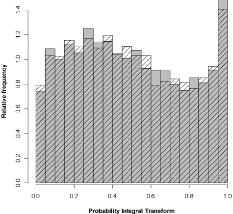
Forecast reliability measures assess the statistical consis-tency of the forecast probability distributions and the ob-served frequency of associated events (Toth et al., 2003). For this study we use histograms of probability integral trans-forms (PIT) to assess the average reliability of the forecast probability distributions for all locations and seasons.

3 Catchments and data

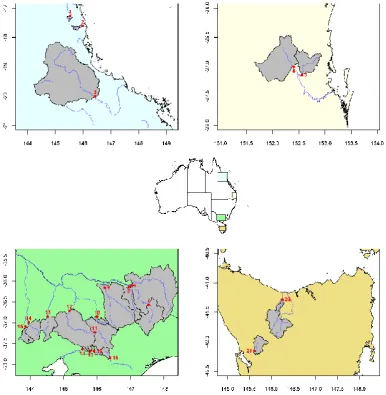
In this study, we investigate the performance of forecasts made using the two different sets of predictors represent-ing the initial catchment condition for 21 catchments in east-ern Australia that experience a range of climatic and hydro-logical conditions (Figs. 1, 2 and Table 1). We use the ob-served monthly streamflow data obtained from various wa-ter resource management agencies and the Bureau of Mete-orology. For most catchments, with the exception of some in Queensland and Victoria, the data are available from 1950 to 2008 (see Table 1). The monthly catchment average rainfall and potential evapotranspiration for each catchment are cal-culated from 5 km gridded data available from the Australian Water Availability Project (Jones et al., 2009). The monthly values of the 13 climate indices are obtained from the Bureau of Meteorology and described in Appendix A.

4 Results

4.1 Forecast skill improvements

Fig. 1. Location of study catchments (location numbers correspond to identifiers in Table 1).

where the skill of forecasts made using selected predictors is less than 10 %.

Figure 4 presents the increase in forecast skill that is achieved by replacing the selected predictors by the WA-PABA simulations and lag-1 streamflow arranged by catch-ment and season. Increases in both skill scores are most pro-nounced in the Queensland catchments (at the top of Fig. 4) and for the MJJ, JJA, NDJ and DJF seasons in the central Victorian and Upper Murray catchments. Decreases in fore-cast skill are most evident for the MAM and AMJ seasons in central Victorian and Upper Murray catchments. The sea-sons where there is the greatest increase in skill tend to be those that cover the steepest rise or fall of the annual hydro-graph (see Fig. 2) and therefore this suggests that the selected predictors are unable to adequately capture the inter-annual variations in the dynamics of catchments wetting and drying. Figure 5 presents the skill scores of cross validation fore-casts by catchment and season. There is a distinct seasonal

Table 1. Attributes of the 21 catchments used for the study. (Res. indicates Reservoir inflow, HES indicates inflow to hydroelectric scheme).

Mean

annual Annual

Available Catchment rainfall Mean annual runoff

ID Catchment Region Record area (km2) (mm) flow (mm) coeff.

1 Barron River Queensland 1950–2008 228 1367 605 (138 GL) 0.44

2 South Johnstone River Queensland 1974–2008 390 3128 2018 (787 GL) 0.65

3 Burdekin River Queensland 1967–2008 36 260 567 76 (2765 GL) 0.13

4 Brisbane River Queensland 1950–2000 3866 846 79 (304 GL) 0.09

5 Somerset Res. Queensland 1950–2000 1366 1245 289 (395 GL) 0.23

6 Hume Res. Upper Murray 1950–2008 12 184 819 227 (2764 GL) 0.28

7 Dartmouth Res. Upper Murray 1950–2008 3193 1042 279 (890 GL) 0.27

8 Kiewa River Upper Murray 1965–2008 1748 1099 248 (433 GL) 0.23

9 Ovens River Upper Murray 1959–2008 7543 963 175 (1320 GL) 0.18

10 Nillahcootie Res. Central Victoria 1950–2008 422 942 150 (63 GL) 0.16

11 Eildon Res. Central Victoria 1950–2008 3877 1104 373 (1447 GL) 0.34

12 Goulburn Res. Central Victoria 1950–2008 7166 769 188 (1349 GL) 0.24

13 Eppalock Res. Central Victoria 1950–2008 1749 630 98 (172 GL) 0.16

14 Cairn Curran Res. Central Victoria 1950–2008 1603 617 72 (115 GL) 0.12

15 Tullaroop Res. Central Victoria 1950–2008 702 633 77 (54 GL) 0.12

16 Thompson Res. Southern Victoria 1950–2008 487 1299 485 (236 GL) 0.37 17 Upper Yarra Res. Southern Victoria 1950–2008 336 1387 443 (149 GL) 0.32 18 Maroondah Res. Southern Victoria 1950–2008 129 1351 577 (74 GL) 0.43 19 O’Shannassy Res. Southern Victoria 1950–2008 127 1404 766 (97 GL) 0.55

20 Mersey-Forth HES Tasmania 1950–2008 2698 1900 793 (2141 GL) 0.42

21 King HES Tasmania 1950–2008 731 2703 1724 (1260 GL) 0.64

Fig. 2. Plot of streamflow seasonality for all catchments. (Mean an-nual flow is provided following the catchment name).

4.2 Forecast reliability

Replacing the selected predictors representing initial catch-ment conditions with WAPABA simulations and lag-1 streamflow produced little change in the reliability of stream-flow forecasts. Figure 6 presents histograms of the PIT val-ues for forecasts of made using both sets of predictors. The differences between the two histograms are small and the general pattern of the histograms is similar. Perfectly reli-able forecasts will produce a PIT histogram that is a uniform distribution. Figure 6 suggests that when viewed collectively the forecasts are not necessarily reliable, with the most obvi-ous deviations from uniformity occurring in the highest and lowest bins of the histogram. However when the reliability is assessed for each season and catchment separately, devia-tions from uniformity are within the range expected by sam-ple variability.

4.3 Reasons for improvements in forecast skill

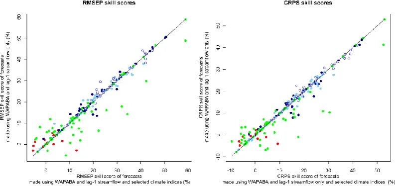
Fig. 3. Skill scores of forecasts made using WAPABA simulations and lag-1 streamflow as predictors plotted against skill scores of forecasts made using selected predictors for the RMSEP (left panel) and CRPS (right panel) skill scores. Each point represents the skill of forecasts for a single location and season. Points above the 1 : 1 line indicate improvements in forecast skill. (Green points are catchments in Queensland, red points are catchments in Tasmania, hollow blue circles tributaries to the upper Murray River, light blue are catchments in central Victoria and dark blue are catchments in southern Victoria).

Fig. 4. Increase in skill scores of forecasts achieved by replacing selected predictors representing initial catchment conditions with WAPABA simulations and lag-1 streamflow.

the historical record. Here we examine some examples of how replacing the selected predictors with WAPABA simula-tions and lag-1 streamflows influences cross-validation fore-casts and improves forecast skill.

4.3.1 When the catchment is wetting up

The selected predictors are either antecedent streamflow or rainfall totals for the previous month. When the catchment is wetting up, antecedent streamflows are primarily base flow and have not necessarily responded to antecedent rain-fall. Therefore, antecedent streamflow does not necessarily

represent the wetness of the catchment well. Where an-tecedent rainfall totals have been insufficient to saturate the catchment, they will primarily reflect the surface moisture conditions of the catchment.

Fig. 5. Skill scores of the cross-validation forecasts made using WAPABA simulations and lag-1 streamflow as predictors.

Fig. 6. Probability Integral Transform histograms illustrating the re-liability of forecasts made using selected predictors (solid grey bars) and WAPABA and lag-1 streamflow as predictors (hatched bars).

initial catchment conditions is predominantly total stream-flow for January and February, which will provided an in-dication of base flow conditions. Overall the forecast quan-tile ranges for a given forecast median are similar using both sets of predictors, however forecast medians are rearranged. By replacing the selected predictors with WAPABA simu-lations and lag-1 streamflow the forecast error is reduced, particularly for forecasts associated with observations in the upper and lower quartiles of the historical distribution (light grey shade in Fig. 6). The primary reason for the differ-ence between the forecasts produced using the two sets of predictors is due to the WAPABA simulations being more

Fig. 7. Forecasts of Kiewa River inflows into the Murray River for the March-April-May season. Using selected predictors, RM-SEP skill score = 9 % and CRPS skill score = 1 %, using WA-PABA simulations and lag-1 streamflow as predictors RMSEP skill score = 18 %, and CRPS skill score = 10 %. (1 : 1 line, forecast me-dian; dark blue vertical line, forecast [0.25, 0.75] quantile range; light and dark blue vertical line, forecast [0.10, 0.90] quantile range; dark grey horizontal line, climatological median; mid-gray shade, climatological [0.25, 0.75] quantile range; light and mid-gray shade, climatological [0.10, 0.90] quantile range; red dot, observed catch-ment inflow).

Fig. 8. Forecasts of inflows into Dartmouth Reservoir for the November-December-January season. Using selected predictors, RMSEP skill score = 19 % and CRPS skill score = 17 %, using WA-PABA simulations and lag-1 streamflow as predictors RMSEP skill score = 31 %, and CRPS skill score = 28 %. (legend as per Fig. 7).

4.3.2 When the catchment is drying out

When the catchment is drying out, antecedent streamflows may be dominated by direct surface runoff if there has been recent rain, or by base flows if there has not been. Total monthly streamflows of similar magnitude can be produced by both sources and therefore antecedent streamflow may not necessarily provide the best indicator of the wetness of a catchment. Figure 8 provides an example of forecasts made for this situation of November-December-January forecasts for inflows into Dartmouth Reservoir. For this example, re-placing the selected predictor representing initial catchment conditions with WAPABA simulations and lag-1 streamflow increases the RMSEP skill score from 19 % to 31 % and the CRPS skill score from 17 % to 28 %. The selected predictor representing initial catchment conditions is predominantly total streamflow for September and October. Like the pre-vious example, when the catchment is wetting up, the fore-cast quantile ranges for a given forefore-cast median are similar using both sets of predictors and the forecast medians are re-arranged. However, in contrast to the previous example, the skill gains are achieved by reducing the errors of the median of forecasts with corresponding observations in the central quartiles (mid-gray shade in Fig. 7) of the historical obser-vations rather than in the outer quartiles. It is for these mod-erate seasonal flow totals that antecedent streamflows could be sourced from either surface runoff or base flow and the WAPABA simulations can distinguish the dominant source, whereas the candidates used in predictor selection cannot. As with the previous example the WAPABA simulations are more strongly correlated to streamflows during the forecast period than any of the candidate predictors representing ini-tial catchment conditions used in the predictor selection.

4.3.3 When the catchment is intermittently saturated

The soil moisture and groundwater stores of a catchment are bounded, that is, soil can become saturated and groundwater

Fig. 9. Forecasts of inflows into Upper Yarra Reservoir for the July-August-September season. Using selected predictors, RMSEP skill score = 5 % and CRPS skill score = 3 %, using WAPABA simula-tions and lag-1 streamflow as predictors RMSEP skill score = 17 %, and CRPS skill score = 12 %. (legend as per Fig. 7).

water tables can approach the surface. However, the an-tecedent streamflow and rainfall totals used as candidate in-dicators of the catchment condition in predictor selection are theoretically unbounded, that is, they continue to increase when the soil moisture and groundwater stores are full. When the soil in a catchment is saturated and groundwater stores are near capacity in the month preceding a forecast, an-tecedent streamflow and rainfall are poor indicators of the condition. For a given forecast period, a catchment may be saturated consistently or intermittently throughout the histor-ical record. For much of the year, the Tasmanian catchments considered in this study provide examples of consistently sat-urated catchment conditions throughout the historical record. For these locations and seasons, the forecast skill is close to zero and replacing the selected predictors with WAPABA simulations and lag-1 streamflow results in little change in forecast skill.

Fig. 10. Relationship between predictors representing initial catch-ment conditions and seasonal streamflow totals for July-August-September inflows into Upper Yarra Reservoir.

with the WAPABA simulations than any of the candidate in-dicators of initial catchment conditions considered in the pre-dictor selection process.

The relationship between streamflow during the forecast period and the WAPABA simulations is approximately lin-ear (Fig. 10). The relationship between streamflows during the forecast period and other variables used as candidates for predictor selection appears linear for low values of the can-didate predictor and deviate from linearity above a threshold value. This two-part relationship suggests that for low values the candidate predictors are reasonable indicators of the ini-tial catchment conditions, but at higher values they are not. Examining the initialised state variables of WAPABA used in producing the simulations that represent initial catchment conditions suggests that when the antecedent streamflows ex-ceed this threshold the soil moisture store is at or near ca-pacity and the groundwater store level is very high. There-fore, the improvements in forecast skill arising from replac-ing the selected predictors with WAPABA simulations and lag-1 streamflow can be attributed to a better representation of the catchment process when the catchment intermittently becomes very wet.

5 Discussion

In this study, selected predictors representing initial catch-ment conditions were replaced by a combination of simula-tions from a dynamic hydrological model and lag-1 stream-flows. Lag-1 streamflows were included as a form of model updating to provide a real-time measure of the actual catch-ment condition leading up to the forecast. However, as lag-1 streamflow is not always a good indicator of the catchment condition and its inclusion may moderate some of the bene-fit of using the WAPABA simulations. Figure 11 presents the increases in forecast skill arising from using lag-1 stream-flows as well as WAPABA simulations to represent the initial catchment condition. In general, including lag-1 streamflow to provide a real-time measure of the actual catchment condi-tion has little impact on the forecast skill. In some instances,

including lag-1 streamflow increases forecast skill for a small number of seasons and locations, but most importantly it does not degrade forecast skill. Therefore, it appears that in-cluding lag-1 streamflows as a form of model update is ap-propriate.

For this study, we simulated the initial catchment influ-ence on future streamflows by forcing initialised hydrologi-cal models with monthly climatology mean rainfall and po-tential evapotranspiration. Our motivation for using simu-lated streamflows, rather than the state variables from WA-PABA, was because the simulated streamflows integrate the condition of both the model soil moisture and groundwater stores. The relative influence of soil moisture and ground wa-ter levels on seasonal streamflows varies with forecast date. Examples of this seasonally varying relationship are shown in Figs. 13 and 14. For forecasts made at the start of May, the May-June-July streamflow totals are more highly correlated with the groundwater storage levels than the soil moisture, or lag-1 streamflow (Fig. 13). For forecasts made at the start of November, November-December-January streamflow totals are more highly correlated with soil moisture than ground-water storage levels, or lag-1 streamflow (Fig. 14). In both instances, the correlation between the WAPABA simulations and the seasonal streamflow totals are comparable to the bet-ter of the two state variables. Therefore, the WAPABA sim-ulations appear to be robust representations of the integrated condition of both the soil moisture and groundwater stores at the forecast time.

For the majority of catchments and seasons, the skill of forecasts is due to the knowledge of the initial catchment condition. Figure 12 illustrates the contribution of the climate indices to forecast skill. When the points in Fig. 12 are lo-cated on the 1 : 1 line the climate indices make no contribu-tion to the skill of streamflow forecasts, while points below the 1 : 1 line suggest that climate indices improve forecast skill. The contribution of climate indices to streamflow fore-cast skill tends to be largest for catchments in Queensland, where there is the strongest evidence for using climate in-dices to forecast seasonal rainfall (Schepen et al., 2012).

The points above the 1 : 1 line in Fig. 12 indicate that fore-casts made without selected climate indices are more skilful that those made with climate indices. This suggests that while there is evidence for using climate indices to forecast rainfall during a fitting period, the fitted relationship does not per-form well for independent forecasts. The approach to assess-ing forecast skill used in this paper is designed to expose cir-cumstances where this occurs and assess the true skill of the predictor selection and forecasting approaches by using cross validated predictors as well as cross-validated model param-eters. Where the predictors are not cross validated, it is likely that the reported forecast skill is artificially inflated and will not be maintained in operational applications (Michaelsen, 1987; DelSole and Shukla, 2009).

Fig. 11. Increase in skill scores of forecasts achieved by using lag-1 streamflow as well as WAPABA simulations to represent the initial catchment condition.

Fig. 12. The contribution of selected climate indices to forecast skill illustrated by plotting skill scores of forecasts made without using climate indices as predictors against skill scores of forecasts made with selected climate indices as predictors for the RMSEP (left panel) and CRPS (right panel) skill scores. All forecasts use WAPABA simulations and lag-1 streamflows as predictors to represent the influence of initial catchment conditions. (Legend as per Fig. 3)

this approach to limit the potential for forecast performance to be artificially inflated due to the state variables in WA-PABA carrying information from one time step to the next and resulting in forecasts that are not independent of data used for parameter inference. We tested the assumption that leave-one-plus-four-years-out was sufficient to create independent forecasts by also assessing forecast skill us-ing leave-one-plus-one-years-out and leave-one-plus-nine-years-out. In the assessment, we fixed the climate predic-tors so that variations in the forecast performance measures were solely due to the different periods omitted from the data used for parameter inference. The differences between the

forecast skill scores produced using the different cross vali-dation methods tended to be within the range of sample vari-ability (not shown). Where there were differences there was no clear pattern to the best or worst performing cross vali-dation approach and therefore the adopted approach appears appropriate.

Fig. 13. The relationship between May-June-July streamflow to-tals and the WAPABA state variables at the end of April. April streamflow and WAPABA simulations for May-June-July for Kiewa River inflows into the Murray River (Pearson correlation coeffi-cients shown in top left corner of each plot).

Many dynamic coupled ocean–atmosphere models have been developed to produce seasonal climate forecasts (for exam-ple: Alves et al., 2002). These models simulate the dynamic evolution of chaotic ocean and atmospheric processes from estimates of the ocean, atmosphere and land surface initial conditions. Forecasts of rainfall, or other atmospheric vari-ables, produced by these models may provide better indica-tors of future climate influences on seasonal streamflows than simple climate indices because they integrate a wide range of initial conditions. They also provide the opportunity for the use of concurrent relationships, which tend to be stronger than lagged relationships. However, comprehensive analysis of dynamic climate model output is necessary to better un-derstand the quality of the forecasts and which variables are useful for streamflow forecasting. Future work will investi-gate using forecasts from dynamic climate models for sea-sonal forecasting of streamflows in Australia using statistical models and rainfall–runoff models.

WAPABA simulates monthly streamflow totals in valida-tion periods using monthly forcing data, as well as daily rainfall–runoffs models forced with daily data (Wang et al., 2011). However, the skill of raw WAPABA simulations rep-resenting the initial catchment condition was considerably poorer than the forecasts resulting from using the WAPABA simulations as a predictor in the BJP modelling approach. The poor skill of the raw WAPABA simulations represent-ing initial catchment condition is primarily due to variation

Fig. 14. The relationship between November-December-January streamflow totals and the WAPABA state variables at the end of October. October streamflow and WAPABA simulations for November-December-January for Kiewa River inflows into the Murray River (Pearson correlation coefficients shown in top left corner of each plot).

in seasonal biases than overall forecast performance measure do not diagnose (not shown). The BJP modelling approach was able to extract information from the biased WAPABA simulations and produce skilful forecasts with minimal bi-ases. The water balance model used in this study is a rela-tively simple, lumped monthly model. Situations may exist where such a model may not necessarily provide sufficient spatial, temporal or process resolution to adequately describe the catchment condition at the forecast time. In these situa-tions, more sophisticated models may be warranted to de-scribe the catchment conditions. Simulations from more so-phisticated models can also be included as predictors in the BJP modelling approach using the process described in this paper.

6 Conclusions

Table A1. Climate indices included as candidate predictors of seasonal forecast of streamflow and data sources.

Period of

Candidate predictors record used Data source

Southern Oscillation Index (SOI) (Troup, 1965) 1950–2008 Australian Bureau of Meteorology NINO3 (SST anomaly over 90◦W–150◦W, 5◦S–5◦N) 1950–2008 NCAR, ERSST.v3 (Smith et al., 2008) NINO3.4 (SST anomaly over 120◦W–170◦W, 5◦S–5◦N) 1950–2008 NCAR, ERSST.v3 (Smith et al., 2008) NINO4 (SST anomaly over 150◦W–160◦E, 5◦S–5◦N) 1950–2008 NCAR, ERSST.v3 (Smith et al., 2008) ENSO Modoki Index (Ashok et al., 2003) 1950-2008 NCAR, ERSST.v3 (Smith et al., 2008) 20◦Isotherm (Ruiz et al., 2006) 1980–2008 Bureau of Meteorology

Indian Ocean Dipole Mode Index (Saji et al., 1999) 1950-2008 NCAR, ERSST.v3 (Smith et al., 2008) Indian Ocean West Pole Index (Saji et al., 1999) 1950–2008 NCAR, ERSST.v3 (Smith et al., 2008) Indian Ocean East Pole Index (Saji et al., 1999) 1950–2008 NCAR, ERSST.v3 (Smith et al., 2008) Indonesia Index (Verdon and Franks, 2005) 1950-2008 NCAR, ERSST.v3 (Smith et al., 2008) Tasman Sea Index (Murphy and Timbal, 2008) 1950–2008 NCAR, ERSST.v3 (Smith et al., 2008) Southern Annular Mode (Marshall, 2003) 1979–2008 Antarctic Oscillation Index NOAA (Mo, 2000)

140◦E Blocking Index (Risbey et al., 2009) 1950–2008 Calculated from NCEP/NCAR reanalysis data (Kalnay et al., 1996)

forecasting, but often require statistical post-processing to remove biases and correct the reliability of forecast prob-ability distributions. This study has investigated whether a hybrid seasonal forecasting system that uses the output of a dynamic hydrological model as a predictor in a statisti-cal forecasting approach can lead to more skilful forecasts. Forecasts of three month streamflow totals were made using two alternative sets of predictors to represent initial catch-ment conditions: predictors selected using the method em-ployed in the operational practice by the Bureau of Meteorol-ogy in Australia; and the combination of simulations from a monthly water balance model that represents the influence of initial catchment condition of streamflows and lag-1 stream-flow. The skill and reliability of streamflow forecasts made using these sets of predictors were compared for 21 catch-ments in eastern Australia and insights into the reasons for any differences investigated.

In general, replacing selected predictors representing the initial catchment condition with simulations from a monthly balance model and lag-1 streamflow increases the forecast skill and has little impact on forecast reliability. The mag-nitude of the skill increases varies with location and season. The greatest increases in forecast skill tend to be for three sets of circumstances: (1) when the catchment is wetting up but antecedent streamflows have not responded to antecedent rainfall; (2) when the catchment is drying and the dominant source of antecedent streamflow is in transition between sur-face runoff and base flow; and (3) when the initial catch-ment condition is near saturation intermittently throughout the historical record. There is little change in forecast skill for catchments and seasons that are very dry or consistently satu-rated throughout the historical record. Even with the skill im-provements realised by replacing the selected predictors, the skill of streamflow forecasts tends to be the highest for sea-sons that include the falling limb of the annual hydrograph, when seasonal streamflows are strongly related to the ini-tial catchment condition. The skill tends to be the lowest for

seasons that include the rising limb, when seasonal stream-flows are strongly related to concurrent rainfall. In general the contribution of climate indices used to represent the in-fluence of future climate to forecast skill is small but compa-rable to that of forecasts of seasonal rainfall. Future work will investigate how using the output of dynamic climate models may improve this situation.

Lag-1 streamflow was included as a predictor in addition to the monthly water balance simulations as a form of model updating to provide a real-time measure of the catchment condition. In general, it contributes little to forecast skill, but for some seasons and location skill increases of up to 20% are realised by its inclusion. Most importantly, including lag-1 streamflow does not degrade forecast skill and therefore can be confidently included as a predictor for operational fore-casts. The use of a more sophisticated hydrological model with increased spatial, temporal or process resolution may reduce the need for model updating. The output of such a higher resolution hydrological model could be used as a pre-dictor in the BJP modelling approach using the methods de-scribed in this paper.

Appendix A

Climate indices used as candidate predictors

Climate indices used as candidate predictors to represent the influence of climate during the forecast period on stream-flows.

Supplementary material related to this article is

Acknowledgements. This research has been supported by the Water Information Research and Development Alliance between the Australian Bureau of Meteorology and CSIRO Water for a Healthy Country Flagship, the South Eastern Australian Climate Initiative, and the CSIRO OCE Science Leadership Scheme. We would like to thank Jeff Perkins, Senlin Zhou, Andrew Schepen, Trudy Wilson and Daehyok Shin from the Australian Bureau of Meteorology for many valuable discussions, as well as providing the rainfall and climate index data for this study. Streamflow and GIS data were provided by the Murray–Darling Basin Authority, Melbourne Water, HydroTasmania, Goulburn-Murray Water, the Australian Bureau of Meteorology and the Queensland Department of Environment and Resource Management.

Edited by: M. Werner

References

Alves, O., Wang, G., Zhong, A., Smith, N., Tzeitkin, F., Warren, G., Schiller, A., Godfrey, S., and Meyers, G.: POAMA: Bureau of Meteorology Operational Coupled Model Seasonal Forecast System, National Drought Forum, Brisbane, 2002.

Ashok, K., Guan, Z. Y., and Yamagata, T.: Influence of the Indian Ocean Dipole on the Australian winter rainfall, Geophys. Res. Lett., 30, doi:10.1029/2003GL017926, 2003.

Bierkens, M. F. P. and van Beek, L. P. H.: Seasonal Predictability of European Discharge: NAO and Hydrological Response Time, J. Hydrometeorol., 10, 953–968, doi:10.1175/2009jhm1034.1, 2009.

DelSole, T. and Shukla, J.: Artificial Skill due to Predictor Screen-ing, J. Climate, 22, 331–345, doi:10.1175/2008jcli2414.1, 2009. Duan, Q., Sorooshian, S., and Gupta, V. K.: Optimal use of the SCE-UA global optimization method for calibrating watershed mod-els, J. Hydrol., 158, 265–284, 1994.

Garen, D. C.: Improved Techniques in Regression-Based Stream-flow Volume Forecasting, J. Water Resour. Pl.-ASCE, 118, 654– 670, doi:10.1061/(ASCE)0733-9496(1992)118:6(654), 1992. Jolliffe, I. T. and Stephenson, D. B.: Forecast verification: a

prac-titioner’s guide in atmospheric science, J. Wiley, Chichester, 240 pp., 2003.

Jones, D. A., Wang, W., and Fawcett, R.: High-quality spatial cli-mate data-sets for Australia, Aust. Meteorol. Oceanogr. J., 58, 233–248, 2009.

Kalnay, E., Kanamitsu, M., Kistler, R., Collins, W., Deaven, D., Gandin, L., Iredell, M., Saha, S., White, G., Woollen, J., Zhu, Y., Chelliah, M., Ebisuzaki, W., Higgins, W., Janowiak, J., Mo, K. C., Ropelewski, C., Wang, J., Leetmaa, A., Reynolds, R., Jenne, R., and Joseph, D.: The NCEP/NCAR 40-year reanalysis project, B. Am. Meteorol. Soc., 77, 437–471, 1996.

Koster, R. D., Mahanama, S. P. P., Livneh, B., Lettenmaier, D. P., and Reichle, R. H.: Skill in streamflow forecasts derived from large-scale estimates of soil moisture and snow, Nat. Geosci., 3, 613–616, 2010.

Marshall, G. J.: Trends in the southern annular mode from observations and reanalyses, J. Climate, 16, 4134–4143, doi:10.1175/1520-0442(2003)016<4134:TITSAM>2.0.CO;2, 2003.

Michaelsen, J.: Cross-validation in statistical climate forecast mod-els, J. Clim. Appl. Meteorol., 26, 1589–1600, 1987.

Mo, K. C.: Relationships between low-frequency variability in the Southern Hemisphere and sea surface temperature anomalies, J. Climate, 13, 3599–3610, doi:10.1175/1520-0442(2000)013<3599:RBLFVI>2.0.CO;2, 2000.

Murphy, B. F. and Timbal, B.: A review of recent climate variability and climate change in southeastern Australia, Int. J. Climatol., 28, 859–879, doi:10.1002/joc.1627, 2008.

Nash, J. E. and Sutcliffe, J. V.: River flow forecasting through con-ceptual models part I – A discussion of principles, J. Hydrol., 10, 282–290, doi:10.1016/0022-1694(70)90255-6, 1970.

Pagano, T. C., Garen, D. C., Perkins, T. R., and Pasteris, P. A.: Daily Updating of Operational Statistical Seasonal Water Supply Fore-casts for the western US, J. Am. Water Resour. As., 45, 767–778, doi:10.1111/j.1752-1688.2009.00321.x, 2009.

Plummer, N., Tuteja, N. K., Wang, Q. J., Wang, E., Robertson, D. E., Zhou, S., Schepen, A., Alves, O., Timbal, B., and Puri, K.: A seasonal water availability prediction service: Opportu-nities and Challenges, 18th World IMACS/MODSIM Congress, Cairns, 13–17 July 2009.

Risbey, J. S., Pook, M. J., McIntosh, P. C., Wheeler, M. C., and Hendon, H. H.: On the Remote Drivers of Rainfall Vari-ability in Australia, Month. Weather Rev., 137, 3233–3253, doi:10.1175/2009mwr2861.1, 2009.

Robertson, D. E. and Wang, Q. J.: A Bayesian approach to predictor selection for seasonal streamflow forecasting, J. Hydrometeorol., 13, 155–171, 2012.

Rosenberg, E. A., Wood, A. W., and Steinemann, A. C.: Statisti-cal applications of physiStatisti-cally based hydrologic models to sea-sonal streamflow forecasts, Water Resour. Res., 47, W00H14, doi:10.1029/2010wr010101, 2011.

Ruiz, J. E., Cordery, I., and Sharma, A.: Impact of mid-Pacific Ocean thermocline on the prediction of Australian rainfall, J. Hy-drol., 317, 104–122, doi:10.1016/j.jhydrol.2005.05.012, 2006. Saji, N. H., Goswami, B. N., Vinayachandran, P. N., and Yamagata,

T.: A dipole mode in the tropical Indian Ocean, Nature, 401, 360– 363, 1999.

Schepen, A., Wang, Q. J., and Robertson, D. E.: Evidence for using climate indices to forecast Australian seasonal rainfall, J. Cli-mate, 25, 1230–1246, 2012.

Shi, X., Wood, A. W., and Lettenmaier, D. P.: How Essen-tial is Hydrologic Model Calibration to Seasonal Stream-flow Forecasting?, J. Hydrometeorol., 9, 1350–1363, doi:10.1175/2008JHM1001.1, 2008.

Smith, T. M., Reynolds, R. W., Peterson, T. C., and Lawrimore, J.: Improvements to NOAA’s historical merged land-ocean surface temperature analysis (1880–2006), J. Climate, 21, 2283–2296, doi:10.1175/2007jcli2100.1, 2008.

Toth, Z., Talagrand, O., Candille, G., and Zhu, Y.: Probability and Ensemble Forecasts, in: Forecast Verification: A Practitioner’s Guide in Atmospheric Science, edited by: Jolliffe, I. T. and Stephenson, D. B., J. Wiley, Chichester, 137–164, 2003. Troup, A. J.: Southern oscillation, Q. J. Roy. Meteorol. Soc., 91,

390, doi:10.1002/qj.49709139009, 1965.

Verdon, D. C. and Franks, S. W.: Indian Ocean sea surface tem-perature variability and winter rainfall: Eastern Australia, Water Resour. Res., 41, W09413, doi:10.1029/2004WR003845, 2005. Wang, Q. J. and Robertson, D. E.: Multisite probabilistic forecasting

Wang, Q. J., Robertson, D. E., and Chiew, F. H. S.: A Bayesian joint probability modeling approach for seasonal forecasting of streamflows at multiple sites, Water Resour. Res., 45, W05407, doi:10.1029/2008WR007355, 2009.

Wang, Q. J., Pagano, T. C., Zhou, S. L., Hapuarachchi, H. A. P., Zhang, L., and Robertson, D. E.: Monthly versus daily water balance models in simulating monthly runoff, J. Hydrol., 404, 166–175, 2011.

Wang, Q. J., Shrestha, D. L., Robertson, D. E., and Pokhrel, P.: A log-sinh transformation for data normalization and variance stabilization, Water Resour. Res., 48, W05514, doi:10.1029/2011wr010973, 2012.

Wood, A. W. and Schaake, J. C.: Correcting Errors in Streamflow Forecast Ensemble Mean and Spread, J. Hydrometeorol., 9, 132– 148, doi:10.1175/2007JHM862.1, 2008.

Wood, A. W., Kumar, A., and Lettenmaier, D. P.: A retrospec-tive assessment of National Centers for Environmental Predic-tion climate model-based ensemble hydrologic forecasting in the western United States, J. Geophys. Res.-Atmos., 110, D04105, doi:10.1029/2004jd004508, 2005.