https://doi.org/10.5194/hess-21-3557-2017 © Author(s) 2017. This work is distributed under the Creative Commons Attribution 3.0 License.
Incorporating remote sensing-based ET estimates into the
Community Land Model version 4.5
Dagang Wang1,2,3,4, Guiling Wang4, Dana T. Parr4, Weilin Liao1,2, Youlong Xia5, and Congsheng Fu4 1School of Geography and Planning, Sun Yat-sen University, Guangzhou, P.R. China
2Guangdong Key Laboratory for Urbanization and Geo-simulation, Sun Yat-sen University, Guangzhou, P.R. China
3Key Laboratory of Water Cycle and Water Security in Southern China of Guangdong High Education Institute, Sun Yat-sen University, Guangzhou, P.R. China
4Department of Civil and Environmental Engineering, University of Connecticut, Storrs, USA
5National Centers for Environmental Prediction/Environmental Modeling Center, and I. M. System Group at NCEP/EMC, College Park, Maryland, USA
Correspondence to:Dagang Wang ([email protected]) and Guiling Wang ([email protected]) Received: 31 December 2016 – Discussion started: 4 January 2017
Revised: 13 June 2017 – Accepted: 13 June 2017 – Published: 14 July 2017
Abstract. Land surface models bear substantial biases in simulating surface water and energy budgets despite the con-tinuous development and improvement of model parame-terizations. To reduce model biases, Parr et al. (2015) pro-posed a method incorporating satellite-based evapotranspi-ration (ET) products into land surface models. Here we ap-ply this bias correction method to the Community Land Model version 4.5 (CLM4.5) and test its performance over the conterminous US (CONUS). We first calibrate a rela-tionship between the observational ET from the Global Land Evaporation Amsterdam Model (GLEAM) product and the model ET from CLM4.5, and assume that this relationship holds beyond the calibration period. During the validation or application period, a simulation using the default CLM4.5 (“CLM”) is conducted first, and its output is combined with the calibrated observational-vs.-model ET relationship to de-rive a corrected ET; an experiment (“CLMET”) is then con-ducted in which the model-generated ET is overwritten with the corrected ET. Using the observations of ET, runoff, and soil moisture content as benchmarks, we demonstrate that CLMET greatly improves the hydrological simulations over most of the CONUS, and the improvement is stronger in the eastern CONUS than the western CONUS and is strongest over the Southeast CONUS. For any specific region, the de-gree of the improvement depends on whether the relationship between observational and model ET remains time-invariant
(a fundamental hypothesis of the Parr et al. (2015) method) and whether water is the limiting factor in places where ET is underestimated. While the bias correction method improves hydrological estimates without improving the physical pa-rameterization of land surface models, results from this study do provide guidance for physically based model development effort.
1 Introduction
(Spenne-mann and Saulo, 2015), analyzing soil moisture variability (Cheng et al., 2015), studying the impact of soil moisture on dust outbreaks (Kim and Choi 2015), and improving the data quality of in situ soil moisture observations (Dorigo et al., 2013; Xia et al., 2015). These model-based estimates of land surface fluxes and state variables are considered an important surrogate for observations, as observational data for some components of the global water and energy cycles are scarce in many regions of the world, and lack spatial and temporal continuity where they do exist. However, land surface models are subject to large uncertainties. Haddeland et al. (2011) compared 11 models in simulating evapotranspi-ration (ET), and found that the global ET on the land surface ranges from 415 to 586 mm yr−1and that the runoff ranges from 290 to 457 mm yr−1. Xia et al. (2012a, b, 2016a, b) doc-umented a large disparity among the four models in NLDAS phase 2 (NLDAS-2) at both the continental and basin scales, and showed that the Mosaic and Sacramento Soil Moisture Accounting (SAC-SMA) models tend to overestimate ET whereas the Noah and Variable Infiltration Capacity (VIC) models tend to underestimate ET.
Great efforts have been made to improve model perfor-mance over the years, by enhancing both the model param-eterization of land surface processes and the model input data. For instance, during the past 10 years, the Community Land Model (CLM) has been upgraded from version 2 to ver-sion 4.5 (Bonan et al., 2002; Oleson et al., 2008, 2013), ac-companied by increasingly accurate and high-resolution sur-face datasets (Lawrence et al., 2011). Comparison with ob-servations of runoff, evapotranspiration, and total water stor-age demonstrated continuous improvement of the model per-formance (Lawrence et al., 2011). The Noah model is an-other example of a continuous upgrade from its original ver-sion since the 1980s (Mahrt et al., 1984). Recent model de-velopments were on vegetation canopy energy balance, the layered snowpack, frozen soil and infiltration, soil moisture– groundwater interaction and related runoff production, and vegetation phenology (Niu et al., 2011). Despite the im-proved understanding and parameterization of physical pro-cesses and better input data, substantial model biases remain (e.g., Parr et al., 2016; Wang et al., 2016).
Another approach to improving model simulations or pre-dictions is through data assimilation, by merging observa-tional data and land surface models to obtain optimal esti-mates for the next time step. Fusing soil moisture observa-tions into land surface models is a typical practice in land data assimilation, and it has been reported that data assimi-lation of soil moisture helped in reducing model biases (Re-ichle and Koster, 2005; Kumar et al., 2008; Yin et al., 2015). However, data assimilation is a computationally intensive task, especially when implementing a multi-model ensemble approach. Moreover, the data assimilation approach is not ap-plicable to future prediction. Parr et al. (2015) proposed an alternative approach to reducing model biases, and applied it to the Variable Infiltration Capacity (VIC) model over the
Connecticut River Basin for both historical simulations and future projections. The Parr et al. (2015) approach assumes that the relationship between the model evapotranspiration (ET) and observational ET remain unchanged from one pe-riod to another, and hence the relationship estimated from the calibration period can be used to correct ET biases and their effects on other variables for any period, historically or in the future. When applied to VIC over the Connecticut River Basin, Parr et al. (2015) found that the ET bias cor-rection approach significantly reduces systematic biases in the estimates of both historical ET and historical river flow, and qualitatively influences the projected future changes in drought and flood risks.
To establish the robustness of the Parr et al. (2015) method, it needs to be evaluated over different regions and differ-ent climate regimes based on differdiffer-ent models. In this study, we implement the Parr et al. (2015) approach in CLM4.5 and evaluate its performance over the whole conterminous United States (CONUS). The land surface model, study area, and bias correction method are introduced in Sect. 2. The data for model calibration and validation, including datasets of ET, runoff, and soil moisture, are described in Sect. 3. Sec-tion 4 presents the calibraSec-tion and validaSec-tion results. Finally, the main findings are summarized and discussed in Sect. 5.
2 Model and methodology 2.1 Model and forcing data
is chosen as the study domain over the globe for the high quality of atmospheric forcing data in this region.
2.2 Methodology
The division of the CONUS into Northwest, Southwest, Northeast, and Southeast, which is based on the 40◦N lat-itude line and the 98◦W longitude line, was defined by Lohmann et al. (2004). This division was later adopted by Xia et al. (2012a) and Tian et al. (2014) when land surface models were evaluated over the CONUS. We follow this di-vision in this study, as shown in Fig. 1a.
Although land surface models are capable of capturing the large-scale pattern of ET, significant biases were found at finer spatiotemporal scales (Parr et al., 2015, 2016; Wang et al., 2016), which propagate to influence other components of the hydrological cycle including runoff and soil moisture (Parr et al., 2015). Following Parr et al. (2015), we derived the climatology of modeled ET for each model grid cell and for each month based on a simulation during the calibration period and climatology of observational ET from satellite-based ET data at the same spatiotemporal resolution during the same period, and estimate the scaling factor between ob-servational ET and the model ET. This scaling factor, which has its unique spatial variability and seasonal cycle, is as-sumed to be time-invariant at the inter-annual and longer timescales. To correct the ET biases in model simulations during any period, two types of simulations are conducted sequentially. In the first type of simulation, named the CLM, we run the default CLM4.5 and save the output for three com-ponents of ET, i.e., interception loss, plant transpiration, and soil evaporation, at the PFT level for every time step. The corrected interception loss, plant transpiration, and soil evap-oration are then derived by multiplying the simulated values by the ET scaling factor, and will be used as the input for the second type of simulation, named CLMET. In CLMET, we re-run CLM4.5 for the same period as in the first type, but overwrite the three ET components simulated by the model with the corrected values. Since ET simulations affect the partitioning of precipitation between ET and runoff, the bias correction in ET is expected to have a direct positive impact on runoff generation and therefore soil moisture.
In this study, we use 1986–1995 as the calibration period and 2000–2014 as the validation period. The simulations dur-ing the calibration period are obtained from a 16-year (1980– 1995) CLM run with the first 6-year run disregarded as the spinup. Both CLM and CLMET runs during the validation period start with the initial condition of 1 January 1996 ob-tained from the calibration period. The time step for both CLM and CLMET runs is 1 h. Since the overwriting process in CLMET may break the water balance, the model checks whether the amount of water stored in the vegetation canopy is sufficient to sustain the interception loss and whether the surface soil water storage is sufficient to sustain soil evapo-ration through the model time step. If not, the interception
loss (soil evaporation) rate is set to be equal to the water available in the vegetation canopy (soil) divided by the model time step. This adjustment minimizes the imbalance caused by overwriting ET components in CLMET.
In this study, the statistics bias, relative bias, and root mean square error (RMSE) are used to validate models in reproduc-ing the spatial pattern against the reference dataset. They are defined as
Bias= 1 N
i=N
X
i=1
Si−Ri, (1)
Relative bias= 1 N
i=N
X
i=1
Si−Ri
Ri , (2) RMSE= v u u u t
i=N
P
i=1
Si−Ri
2
N , (3)
whereN is the total number of grid cells, andSi(Ri)are the temporal average of the model simulated (reference) value for grid celli, which is calculated as
Si= 1
M
j=M
X
j=1
Si,j, (4)
Ri= 1
M
j=M
X
j=1
Ri,j, (5)
whereSi,j(Ri,j)is the model simulated (reference) value at timej and grid celli, andM is the total number of time points. The statistic RMSE is also used to validate models in reproducing time series whereMbecomes the total number of grid cells andN the total number of time points.
3 Data 3.1 ET
3.1.1 GLEAM ET
Figure 1. (a)Mean annual (1980–2015) precipitation in millimeters over the conterminous USA (CONUS). NW, SW, NE, and SE rep-resent the Northwest, Southwest, Northeast, and Southeast CONUS, respectively. The black circles reprep-resent sites of in situ soil moisture observations in Alabama, Illinois, Mississippi, Nebraska, and Oklahoma.(b)Locations of the 16 AmeriFlux stations with vegetation types.
used in studying soil moisture–temperature coupling (Mi-ralles et al., 2012), the impact of land surface on precipitation (Guillod et al., 2015), and the climate control on land surface evaporation (Miralles et al., 2014). Recent evaluations con-ducted at both flux tower site and global scales show that GLEAM-based ET is superior to MODIS-based and Surface Energy Balance System (SEBS) based ET products (Michel et al., 2016; Miralles et al., 2016). The spatial resolution of the GLEAM dataset is 0.25◦, which is consistent with the resolution of CLM4.5 used in this study. The temporal res-olution of the GLEAM dataset is daily, and the monthly ag-gregated ET is used to derive the scaling factors.
3.1.2 MODIS and FLUXNET-MTE ET
Two other gridded ET products are used for independent evaluations: MODIS ET and FLUXNET-MTE (model tree
ensemble) ET. Mu et al. (2007, 2011) produced a MODIS-based global ET dataset using a revised Penman–Monteith (PM) equation. The dataset is arguably the most widely used remote sensing-based global ET product (Miralles et al., 2016). Monthly versions of the MODIS-based prod-uct at the 0.5◦ spatial resolution are used to validate the model with the bias correction method. The FLUXNET-MTE global ET dataset was derived from 253 FLUXNET eddy covariance towers distributed over the globe using the model tree ensemble (MTE) approach (Jung et al., 2009, 2010). The record gaps of half-hourly eddy covariance fluxes were filled first, and the complete tower-based dataset was then used to train the MTE to produce the monthly global ET dataset at the 0.5◦spatial resolution. The data have been
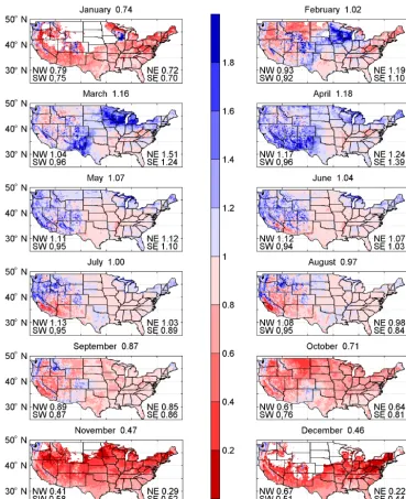
[image:4.612.105.492.65.449.2]Figure 2.Scaling factor as the ratio of the CLM simulated ET to the GLEAM ET for each month during 1986–1995. The numbers in titles are CONUS-averaged values, and the numbers within figures are area-averaged values for each of the four sub-regions (NW, SW, NE, and SE). The areas with negative scaling factors are masked out.
the quality of the FLUXNET-MTE dataset in our study do-main is expected to be good. The MODIS dataset is available for 2000–2014, and the FLUXNET-MTE dataset is available for 1982–2011. We chose the overlap period of these two products, 2000–2011, for model validations using MODIS and the FLUXNET-MTE dataset.
3.1.3 Flux tower ET
ET observations (in energy unit) at 16 sites from the Ameri-Flux network are used to validate the model on the grid cell scale (Fig. 1b). Those sites span four sub-regions (i.e., NW,
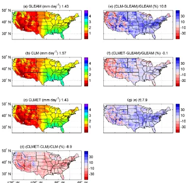
Figure 3.Mean annual ET from(a)GLEAM,(b)the CLM, and(c)CLMET, the relative difference between(d)CLMET and the CLM,
(e)the CLM and GLEAM,(f)CLMET and GLEAM, and(g)the difference between the absolute value of(e)and the absolute value of(f)
during the period 2000–2014. Numbers in titles are CONUS-averaged values.
3.2 Observation-based runoff coefficient
The runoff coefficient (the ratio of runoff to precipitation) of the Global Streamflow Characteristics Dataset (GSCD) ver-sion 1.9 (Beck et al., 2013, 2015) is used to evaluate the model performance in simulating runoff. The GSCD dataset was produced based on streamflow observations from ap-proximately 7500 catchments over the globe. A data-driven approach was adopted to derive the gridded streamflow char-acteristics at the 0.125◦ resolution on a global scale. This
dataset is relatively reliable for the grid cells within which a large number of catchment data are used. The uncertainty is low in North America, Europe, and southeastern Australia, where a large number of observations are available.
3.3 In situ soil moisture observations
The North American Soil Moisture Database (NASMD, Quiring et al., 2016) is used to evaluate the model
Table 1.Spatial evaluations of simulated ET from two different types of runs (CLM and CLMET) against GLEAM-derived ET over the CONUS, Northwest (NW), Southwest (SW), Northeast (NW), and Southeast (SW) annually and seasonally during the period 2000–2014. March–April–May: MAM; June–July–August: JJA; September–October–November: SON; December–January–February: DJF.
Season Region Bias (mm day−1) Relative bias (%) RMSE (mm day−1)
CLM CLMET CLM CLMET CLM CLMET
Annual CONUS 0.137 −0.006 10.8 −0.1 0.266 0.144
NW 0.029 −0.03 7.9 0.3 0.25 0.199
SW 0.074 −0.025 10.2 −3.1 0.181 0.118
NE 0.138 −0.012 9.6 −0.1 0.243 0.132
SE 0.315 0.041 15.6 2.1 0.355 0.099
MAM CONUS −0.081 −0.062 −5.8 −3.3 0.351 0.227 NW −0.138 −0.074 −6.7 −2.7 0.326 0.244 SW −0.211 −0.122 −17.9 −9.3 0.318 0.206 NE −0.191 −0.078 −8.3 −2.8 0.429 0.293
SE 0.19 0.023 8.9 1.5 0.346 0.165
JJA CONUS 0.094 −0.041 6.4 −1.3 0.451 0.331 NW −0.137 −0.121 −3.9 −4.0 0.487 0.408 SW 0.147 −0.006 18.3 −0.9 0.352 0.232
NE 0.045 −0.124 2.5 −2.7 0.55 0.452
SE 0.332 0.075 9.1 2.1 0.414 0.181
SON CONUS 0.360 0.055 51 7.8 0.428 0.155
NW 0.271 0.044 76.4 14.0 0.346 0.147
SW 0.228 0.044 39.5 5.0 0.282 0.117
NE 0.481 0.077 50.4 7.3 0.527 0.242
SE 0.499 0.061 34.5 4.1 0.531 0.11
DJF CONUS 0.182 0.009 77.7 18.9 0.265 0.115
NW 0.114 −0.013 104.2 28.8 0.252 0.122 SW 0.132 −0.014 42.3 −1.9 0.182 0.056
NE 0.239 0.077 146.4 65.3 0.334 0.199
SE 0.24 0.004 49.5 2.7 0.292 0.072
and 50 cm depths for all stations to compare them with the modeled soil moisture for the 0–10 and 0–100 cm layers.
4 Results
4.1 Calibration of ET scaling factor
Figure 2 shows the climatological scaling factors for each month over the CONUS based on the 1986–1995 period. The GLEAM-derived dew and the CLM simulated dew are not consistent in some areas of the Northwest CONUS. If that happens, the scaling factors became negative, because ET is negative for one and positive for the other. We did not scale ET when the scaling factor is negative, and those areas are masked out in Fig. 2. This treatment (scaling in some months and no scaling in other months) may introduce a seasonal bias correction effect in these areas. The model simulations generally agree better with GLEAM estimations during the warm seasons, whereas the difference between simulations and GLEAM estimations remains large during the cold
sea-sons. The scaling factors greatly vary with region. For in-stance, the area-averaged scaling factors for November are 0.34, 0.58, 0.28, and 0.52 for Northwest, Southwest, North-east, and SouthNorth-east, respectively. The overestimation is over-whelming during October, November, December, and Jan-uary, whereas underestimation occurs in many areas during March, April, and May. The overestimation is especially se-vere over the Northeast CONUS where simulated ET is al-most 5 times the GLEAM estimate in December.
4.2 Evaluation
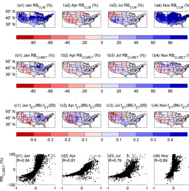
Figure 4. (a)Relative bias (RB) for the CLM (RBCLM),(b)RB for CLMET (RBCLMET) during the period 2000–2014,(c)difference in scaling factorfETbetween the period 1986–1995 and the period 2000–2014 (fET(86)−fET(00)), and(d)scatter plots offET(86)−fET(00) vs. RBCLMETin (1) January (Jan), (2) April (Apr), (3) July (Jul), and (4) November (Nov).
ET are used for validation, we average ET from the four 0.25◦ model grid cells within each 0.5◦ observational grid cell; for the GSCD runoff data, we aggregate observations from 0.125 to 0.25◦to match the model resolution. As in situ
soil moisture observations are technically at the point scale, we spatially average observed soil moisture in each state and compare the averaged observations with the model simula-tions averaged across grid cells within the same state. 4.2.1 ET
Figure 3 shows the multi-year averages (2000–2014) of ET derived from GLEAM, simulated by the CLM and CL-MET, and the relative bias of simulations against GLEAM. Over most of the CONUS, the CLM overestimates ET and CLMET reduces ET as well as ET biases relative to GLEAM data. The averaged relative bias in the CLM over
[image:8.612.109.493.62.449.2]Table 2.Similar to Table 1, but based on comparison with MODIS-derived ET during the period 2000–2011.
Season Region Bias (mm day−1) Relative bias (%) RMSE (mm day−1)
CLM CLMET CLM CLMET CLM CLMET
Annual CONUS 0.321 0.177 30.8 19.1 0.427 0.321
NW 0.28 0.232 35.8 27.9 0.367 0.326
SW 0.282 0.183 39.7 25.6 0.428 0.36
NE 0.278 0.125 19.6 9.1 0.316 0.193
SE 0.431 0.159 24.9 10.6 0.538 0.348
MAM CONUS 0.514 0.533 50.1 55.8 0.631 0.635
NW 0.564 0.628 67.2 74.5 0.636 0.687
SW 0.345 0.438 45.9 61.8 0.538 0.599
NE 0.547 0.655 51.7 61.9 0.58 0.675
SE 0.596 0.436 34.6 25.8 0.735 0.578
JJA CONUS 0.251 0.116 18.2 12.1 0.759 0.691
NW 0.263 0.281 23.8 25.6 0.704 0.71
SW 0.344 0.192 28.8 14.5 0.806 0.724
NE 0.028 −0.144 2.9 −2.4 0.662 0.564
SE 0.31 0.052 13.2 5.8 0.829 0.72
SON CONUS 0.345 0.039 48.2 9.8 0.459 0.284
NW 0.261 0.038 56.8 9.4 0.369 0.261
SW 0.284 0.096 55.9 20.8 0.43 0.306
NE 0.448 0.043 47.4 5.6 0.483 0.207
SE 0.417 −0.019 32.1 2.7 0.547 0.329
DJF CONUS 0.181 0.025 82.2 28 0.383 0.276
NW 0.043 −0.049 77.6 40.4 0.385 0.365
SW 0.156 0.007 70.5 19.4 0.292 0.191
NE 0.091 −0.051 96.7 14.8 0.344 0.214
SE 0.403 0.169 87.5 33.6 0.474 0.281
The improvement from the CLM to CLMET is more sub-stantial for September–October–November (SON) and DJF than MAM and June–July–August (JJA). The relative bias of 51 % (77.7 %) in the CLM is reduced to 7.8 % (18.9 %) in CLMET over the CONUS during SON (DJF). For the re-gional average, the improvement is greatest over the South-east CONUS. All the positive biases in all seasons over the Southeast CONUS are substantially reduced.
To understand the differences between the CLM and CL-MET, we select four months representing each of the four seasons, January, April, July, and November, to examine the relationship between the relative bias of model simulations and the scaling factor changes from the calibration period (1986–1995) to the validation period (2000–2014) in Fig. 4. The improvement from the CLM to CLMET is evident, es-pecially in January and November (Fig. 4a and b). Although the bias is dramatically reduced in CLMET, it remains large in the Northeast CONUS in January (Fig. 4b1). In addition, the bias in CLMET appears larger in the western CONUS than the eastern CONUS (Fig. 4b). The spatial patterns of the relative biases in CLMET and the scaling factor differences between the two periods demonstrate a great degree of
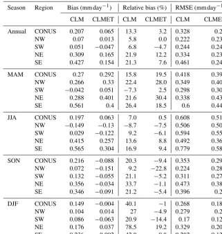
CL-Table 3.Similar to Table 1, but based on comparison with FLUXNET-MTE ET during the period 2000–2011.
Season Region Bias (mm day−1) Relative bias (%) RMSE (mm day−1)
CLM CLMET CLM CLMET CLM CLMET
Annual CONUS 0.207 0.065 13.3 3.2 0.328 0.24
NW 0.07 0.013 5.8 0.0 0.222 0.234
SW 0.051 −0.047 6.8 −4.7 0.244 0.241
NE 0.309 0.165 21.9 12.2 0.334 0.238
SE 0.427 0.154 21.3 7.6 0.461 0.248
MAM CONUS 0.27 0.292 15.8 19.5 0.418 0.399
NW 0.266 0.33 22.4 28.0 0.349 0.401
SW −0.042 0.051 −7.3 2.5 0.298 0.301
NE 0.288 0.401 21.6 30.4 0.338 0.435
SE 0.561 0.4 26.4 18.5 0.6 0.448
JJA CONUS 0.197 0.063 7.0 0.5 0.608 0.517
NW −0.149 −0.13 −8.7 −7.5 0.506 0.506
SW 0.029 −0.122 9.2 −6.1 0.594 0.555
NE 0.415 0.257 13.6 8.8 0.492 0.369
SE 0.565 0.304 16.9 9.4 0.779 0.585
SON CONUS 0.216 −0.088 20.3 −9.4 0.353 0.294 NW 0.072 −0.151 9.2 −22.8 0.224 0.286
SW 0.132 −0.055 21.1 −5.2 0.311 0.277
NE 0.356 −0.034 33.7 −1.1 0.473 0.385
SE 0.346 −0.091 21.2 −5.4 0.396 0.23
DJF CONUS 0.149 −0.004 40.1 −1 0.268 0.189
NW 0.104 0.014 27 −4.9 0.279 0.26
SW 0.086 −0.063 20.9 −14.4 0.17 0.129
NE 0.176 0.037 78.5 19.2 0.329 0.208
SE 0.236 0.002 42.8 0.8 0.282 0.129
MET are greater than in the CLM for the whole CONUS, Northwest, Southwest, and Northeast in MAM. The most considerable improvement occurs in SON compared with the other three seasons. CLMET deteriorates the ET estimate for MAM by enhancing the overestimation already occurring in the CLM, which is different from the validation against the GLEAM-based ET.
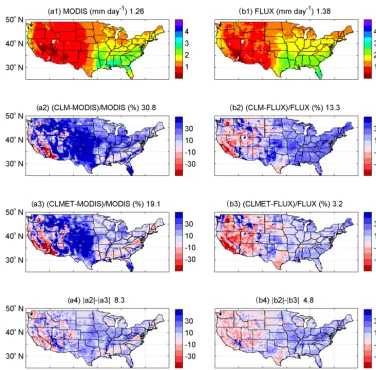
The analysis of time series of ET from MODIS, FLUXNET-MTE, and the two types of simulations also demonstrates improvement from the CLM to CLMET. Cli-matological seasonal cycles of ET over the CONUS and four sub-regions for the period 2000–2011 are shown in Fig. 6. CLMET outperforms the CLM over the CONUS, with a smaller RMSE (0.31 vs. 0.40 against MODIS, 0.19 vs. 0.25 against FLUXNET-MTE). The improvement mainly results from reduction of the overestimation existing in the CLM for SON and DJF. However, the model performance greatly varies with region. As indicated by the ET RMSE values, CL-MET and the CLM perform similarly over some areas of the western CONUS, whereas CLMET improves the ET simula-tion over the eastern CONUS no matter which reference data are used. Figure 7 compares the temporal evolution of the
[image:10.612.137.459.86.426.2]Figure 5.Mean annual ET from(a1)MODIS,(b1)FLUXNET-MTE, the relative differences between(a2)the CLM and MODIS,(b2)
the CLM and FLUXNET-MTE,(a3)CLMET and MODIS, and(b3)CLMET and FLUXNET-MTE, and the differences between(a4)the absolute value of(a2)and the absolute value of(a3), and(b4)the absolute value of(b2)and the absolute value of(b3)during the period 2000–2011. Numbers in titles are CONUS-averaged values.
In addition, the ET validation is also conducted at the site scale (Figs. 8, 9, and 10). Except for Port Peck and Wind River Crane stations in the Northwest CONUS, for all other stations the monthly mean ET from CLMET agrees better with the observed ET than that from the CLM (Fig. 8). The same statement holds for daily mean ET (Figs. 9 and 10). Generally, the CLM overestimates ET as compared with sta-tion observasta-tions, and CLMET alleviates this overestimasta-tion, which is consistent with comparisons between the modelled ET and satellite-based ET products.
4.2.2 Runoff
Using the runoff coefficient (the ratio of runoff to total pre-cipitation) derived from GSCD as the benchmark, we evalu-ate the model performance in the CLM and CLMET in sim-ulating runoff (Fig. 11). The CONUS-averaged runoff coef-ficients in the CLM and CLMET are 0.18 and 0.21, which
are comparable to the GSCD-based runoff coefficient (0.22). However, the CLM underestimates runoff in most areas of the CONUS due to an overestimation of ET. CLMET alle-viates the underestimation by reducing ET, thereby increas-ing the runoff, especially over the eastern CONUS. The rel-ative bias of CLMET against GSCD is 1.1 %, which is much smaller than the value in the CLM (−9.2 %). Table 4 shows the regional difference in runoff simulations in the CLM and CLMET. The improvement is greater over the eastern CONUS than the western CONUS, which is consistent with the improvement of ET simulations. The most striking im-provement occurs in the Southeast CONUS, with the rela-tive bias (RMSE) reduced from−24.7 % (0.091) to−8.2 % (0.06). Because only the multi-year mean annual runoff co-efficient is available for GSCD, we cannot examine the sea-sonal dependency of the model performance improvement.
Figure 6.Seasonal cycles of ET from MODIS, FLUXNET-MTE, the CLM, and CLMET over(a)the CONUS,(b)Northwest,(c)Southwest,
(d)Northeast, and(e)Southeast during the period 2000–2011.
Table 4.Statistics of simulated annual runoff coefficients (ratio of runoff to total precipitation) against GSCD observations over the CONUS, Northwest (NW), Southwest (SW), Northeast (NW), and Southeast (SW) during the period 2000–2014.
Bias Relative bias (%) RMSE
CLM CLMET CLM CLMET CLM CLMET
CONUS −0.053 −0.027 −18.5 −6.7 0.198 0.192 Northwest −0.046 −0.036 −13.5 −5.6 0.146 0.144 Southwest −0.026 −0.019 −19.9 −11.4 0.373 0.373 Northeast −0.06 −0.022 −15.7 −1.5 0.108 0.092 Southeast −0.074 −0.026 −24.7 −8.2 0.091 0.06
same values of the ET scaling factor within each grid cell are applied to three components of ET (interception loss, plant transpiration, and soil evaporation) in this study. Because in-terception loss accounts for a small portion of total ET, the absolute change in interception loss (decrease from the CLM
[image:12.612.157.440.541.636.2]evapo-Figure 7.Time series of ET differences between model (CLM or CLMET) and reference data (MODIS or FLUXNET-MTE) over(a)the CONUS,(b)Northwest,(c)Southwest,(d)Northeast, and(e)Southeast during the period 2000–2011.
ration are more significantly reduced by CLMET, inducing wetter soil and therefore more subsurface runoff.
4.2.3 Soil moisture
As analyzed in Sect. 4.2.2, reductions in all three components of ET interception loss, plant transpiration, and soil evapora-tion from the CLM to CLMET slow down moisture depleevapora-tion from the soil. As a result, the water content in different soil layers increases with reduced ET. Figure 12 shows soil wa-ter at the surface and root-zone layers simulated by the CLM and CLMET, and their differences in August. From the CLM to CLMET, the changes over the CONUS show an over-whelmingly increasing signal for both surface and root-zone soil moisture. The moisture increase in the top 0–100 cm soil layer from the CLM to CLMET in the central CONUS is very evident, which may have significant implications in
drought monitoring and assessment. For example, the Cen-tral Great Plains experienced a severe drought in the summer of 2012, and soil moisture derived from land surface mod-els was used to evaluate the intensity of the drought event (Hoerling et al., 2014; Livneh and Hoerling, 2016). Unfor-tunately, land surface models tend to systematically overes-timate drought (Milly and Dunne, 2016; Ukkol et al., 2016). The more accurate estimates of ET and soil moisture result-ing from the bias correction method in this study may prove useful for improving drought monitoring and assessment.
[image:13.612.128.472.63.465.2]Figure 8.Monthly mean latent heat fluxes from the CLM and CLMET and observations at 16 flux tower sites. RMSECLMand RMSECLMET represent the root mean square error against observations for the CLM and CLMET, respectively. Note that the CLM and CLMET simulations are driven with meteorological forcings at the grid cell level (as opposed to site-specific forcing).
the CLM to CLMET is more evident during SON and DJF, which is consistent with changes in ET that also features more decreases during SON and DJF. The soil in the CLM shows dry biases over most of the examined states, with the exception of soil moisture in the top 10 cm layer in Al-abama and Illinois, and CLMET generally alleviates these dry biases. The RMSE values against the NASMD observa-tions in CLMET are smaller than or at least the same as the RMSE values in the CLM. An exception exists for the top 0–10 cm layer in Alabama and Illinois, where a wet bias is found in the CLM. The soil water content difference between the CLM and CLMET is larger for the 0–100 cm layer than the 0–10 cm layer, because plant transpiration, with which a large fraction of ET and therefore a large fraction of ET
bias correction are associated, primarily depletes moisture from the rooting zone, which is deeper than 10 cm. As such, the improvement is more evident for the top 0–100 cm layer. For example, in Mississippi, the RMSE is reduced from 0.048 m3m−3 in the CLM to 0.042 in CLMET in the top 0–10 cm layer, and from 0.07 to 0.06 m3m−3in the top 0– 100 cm layer. The improvements in Alabama, Mississippi, Nebraska, and Oklahoma are summarized in Table 5.
5 Summary and discussions
Figure 9.Daily mean latent heat fluxes from the CLM and CLMET grids and station observations at ARM SGP Burn, Audubon Grassland, Bondville, Donaldson, Flagstaff Forest, Fort Dix, Fort Peck, and Little Prospect. RMSECLM and RMSECLMET represent the root mean square error against observations for the CLM and CLMET, respectively.
biases over the CONUS. The bias correction algorithm was calibrated using the GLEAM ET product combined with the default CLM4.5 output over the period of 1986–1995, and was validated over the period of 2000–2014 using both grid-ded and site-based ET datasets, the GSCD runoff product, and the NASMD soil moisture data. Results from all evalu-ation metrics indicate improved estimevalu-ation of the terrestrial hydrological cycle across most of the model domain, with different degrees of improvement among the CONUS sub-regions.
as-Figure 10.Daily mean latent heat fluxes from the CLM and CLMET grids and station observations at Mead Rainfed, Metolius Pine, Missouri Ozark, Morgan Forest, Sylvania Wilderness, Tonzi Ranch, Walnut River, and Wind River Crane. RMSECLMand RMSECLMETrepresent the root mean square error against observations for the CLM and CLMET, respectively.
sumption of Parr et al. (2015) (on a time-invariant relation-ship characterizing the default model biases) holds or not. Although the scaling factors between observations and sim-ulations do not change much from the calibration period to the validation period over most regions in most seasons, dra-matic changes do exist in some areas. Differences in the scal-ing factors between the calibration and validation/application periods greatly influence the effectiveness of the bias correc-tion method, with large differences causing the approach to be less effective, leaving substantial biases in CLMET. The
Northeast CONUS during winter is an example of having a large bias in CLMET due to greater changes in the ET scaling factor from the calibration period to the verification period.
[image:16.612.96.501.62.530.2]Figure 11.Mean annual runoff coefficient (the ratio runoff to total precipitation) from(a)the Global Streamflow Characteristics Dataset (GSCD),(b) the CLM, and(c)CLMET, and the relative differences between(d)the CLM and GSCD,(e)CLMET and GSCD, and(f)
CLMET and the CLM during the period 2000–2014. Runoff coefficients of less than 0.02 are blanked out. Numbers in titles are CONUS-averaged values.
corrected at all. All of these three factors (i.e., whether the scaling factor differs significantly between calibration and validation periods, whether ET is underestimated in water-limited regimes, and whether ET scaling is applied at all) in-fluence the effectiveness of the bias correction approach, but one or two of them may dominate for a given region/season. For example, regardless of which product is used as the ref-erence for comparison (Figs. 3g, 5a4, and b4), the approach reduces ET biases over the eastern CONUS where the ET scaling is applied in most places/seasons and the scaling fac-tor shows little difference between the calibration and valida-tion periods. In contrast, in the northern part of the Midwest, some positive biases still remain in CLMET, as the ET scal-ing is not applied in winter months and the scalscal-ing factor differs quite substantially between these two periods. Over some areas of the western CONUS, the bias correction ap-proach is less effective due to the underestimation of ET un-der a water-limited condition and large differences between calibration and validation periods in the scaling factor.
For a given grid cell and given month, the scaling factors for all three ET components, i.e., interception loss, plan tran-spiration, and soil evaporation, are the same in this study, set to be the ratio of the remote sensing ET to the modeled ET. Since the GLEAM dataset contains values of three compo-nents besides the total ET, we conducted additional experi-ments in which the scaling factor for each ET component was
estimated separately, using the ratio of each ET component from the GLEAM product to the corresponding ET compo-nent from the CLM during the same calibration period. How-ever, results based on the component-specific scaling do not show further improvement, which is likely due to the inaccu-rate partitioning of ET into interception loss, plan transpira-tion, and soil evaporation in the GLEAM product. Miralles et al. (2016) compared the ET partitioning for three widely used remote sensing-based ET products, and found that the contribution of each component to ET is dramatically differ-ent among these three products. For instance, they found that the percentage of global ET accounted for by soil evapora-tion ranges from 14 to 52 %, and the ranges are even larger at the regional and local scales. Because the in situ measure-ments of separate components of ET are very scarce, it is par-ticularly challenging to validate the accuracy of the remote sensing-based estimates of the three ET components. These challenges led Miralles et al. (2016) to recommend against the use of any single product in partitioning ET.
pa-Figure 12.Simulated soil moisture (mm) in the top(a)0–10 cm and(b)0–100 cm layers in August from (1) the CLM and (2) CLMET, (3) their differences, and (4) their relative differences during the period 2000–2014.
Table 5.Root mean square error (RMSE) values of monthly vol-umetric soil moisture (m−3m−3) simulated by CLM and CLMET relative to the quality controlled NASMD for the top 0–10 cm soil layer and for the top 0–100 cm soil layer over Alabama, Illinois, Mississippi, Nebraska, and Oklahoma.
top 0–10 cm soil top 0–10 cm soil water content water content
CLM CLMET CLM CLMET
Alabama 0.044 0.048 0.027 0.020 Illinois 0.019 0.021 0.038 0.034 Mississippi 0.048 0.042 0.070 0.060 Nebraska 0.014 0.014 0.032 0.025 Oklahoma 0.050 0.045 0.039 0.032
[image:18.612.65.269.593.699.2]indi-cating a strong potential for performance improvement that can be derived from improving the physical parameteriza-tion of ET processes in the model. Over regions where the bias correction approach does not improve the ET estimate (which are mostly places where ET is water-limited, while the model underestimates ET), parameterizations for other processes that influence soil moisture (e.g., runoff genera-tion, groundwater interactions) are the most likely cause of model biases and should be the focus of physically based model development effort.
Data availability. The GLEAM ET data were provided by the GLEAM team at the website http://www.GLEAM.eu (GLEAM, 2014). The MODIS ET data by NTSG, University of Montana, are at the website http://www.ntsg.umt.edu/project/mod16 (NTSG, 2014). The FLUXNET-MTE ET data were provided by the Max Planck Institute for Biogeochemistry at the website https://www. bgc-jena.mpg.de/geodb/projects/Data.php (Max Planck Institute for Biogeochemistry, 2011). The GSCD runoff data were provided by the Amsterdam Critical Zone Hydrology Group at the web-site http://hydrology-amsterdam.nl/valorisation/GSCD.html (Am-sterdam Critical Zone Hydrology Group, 2010). The original NASMD soil moisture data are available at the website http:// soilmoisture.tamu.edu/ (NASMD, 2012). The quality controlled NASMD soil moisture data can be obtained from the authors upon request. Latent heat flux measurements at the tower sites are avail-able: Flux – http://ameriflux.lbl.gov/ (AmeriFlux network, 2016).
Author contributions. DW and GW designed the study. DW con-ducted model simulations and data analysis with input from GW, DP, and CF. DW and GW wrote the paper with input from YX. WL and YX contributed to data processing.
Competing interests. The authors declare that they have no conflict of interest.
Special issue statement. This article is part of the special issue “Observations and modeling of land surface water and energy ex-changes across scales: special issue in Honor of Eric F. Wood”. It does not belong to a conference.
Acknowledgements. This study is supported by the National Natural Science Foundation of China (grant no. 51379224) and the Fundamental Research Funds for the Central Universities. The authors thank Brecht Martens and two anonymous reviewers for their constructive comments.
Edited by: Niko Verhoest
Reviewed by: Brecht Martens and two anonymous referees
References
Ahmed, M., Sultan, M., Yan, E., and Wahr, J.: Assessing and im-proving land surface model outputs over africa using GRACE, field, and remote sensing data, Surv. Geophys., 37, 1–28, 2016. AmeriFlux network: Latent flux measurements, available at: http:
//ameriflux.lbl.gov/, last access: 31 December 2016.
Amsterdam Critical Zone Hydrology Group: Global streamflow characteristic dataset, multi-year annual average, available at: http://hydrology-amsterdam.nl/valorisation/GSCD.html, 2010. Beck, H. E., Dijk, A. I. J. M., Miralles, D. G., Jeu, R. A. M. D.,
Brui-jnzeel, L. A., Mcvicar, T. R., and Schellekens, J.: Global patterns in base flow index and recession based on streamflow observa-tions from 3394 catchments, Water Resour. Res., 49, 7843–7863, 2013.
Beck, H., De Roo, A., and Van Dijk, A.: Global maps of stream-flow characteristics based on observations from several thousand catchments, J. Hydrometeorol., 16, 1478–1501, 2015.
Bonan, G. B., Oleson, K., Vertenstein, M., Levis, S., Zeng, X., Dai, Y., Dickinson, R., and Yang, Z.: The land surface climatol-ogy of the Community Land Model coupled to the NCAR Com-munity Climate Model, J. Climate, 15, 3123–3149, 2002. Bonan, G. B., Lawrence, P. J., Oleson, K. W., Samuel, L.,
Mar-tin, J., Markus, R., Lawrence, D. M., and Swenson, S. C.: Im-proving canopy processes in the Community Land Model ver-sion 4 (CLM4) using global flux fields empirically inferred from FLUXNET data, J. Geophys. Res.-Biogeo., 116, G2014, https://doi.org/10.1029/2010JG001593, 2011.
Cai, X., Yang, Z. L., Xia, Y., Huang, M., Wei, H., Leung, L. R., and Ek, M. B.: Assessment of simulated water balance from Noah, Noah-MP, CLM, and VIC over CONUS using the NLDAS test bed, J. Geophys. Res.-Atmos., 119, 13751–13770, 2014. Cheng, S., Guan, X., Huang, J., Ji, F., and Guo, R.: Long-term trend
and variability of soil moisture over East Asia, J. Geophys. Res., 120, 8658–8670, 2015.
Dickinson, R. E., Oleson, K., Bonan, G., Hoffman, F. M., Thorn-ton, P., Vertenstein, M., Yang, Z., and Zeng, X.: The Community Land Model and its climate statistics as a component of the com-munity climate system model, J. Climate, 19, 2302–2324, 2010. Dorigo, W. A., Xaver, A., Vreugdenhil, M., Gruber, A., Hegyiová, A., Sanchisdufau, A. D., Zamojski, D., Cordes, C., Wagner, W., and Drusch, M.: Global automated quality control of in situ soil moisture data from the International Soil Moisture Network, Vadose Zone J., 12, 918–924, 2013.
Getirana, A. C. V., Dutra, E., Guimberteau, M., Kam, J., Li, H. Y., Decharme, B., Zhang, Z., Ducharne, A., Boone, A., Balsamo, G., Rodell, M., Toure, A. M., Xue, Y., Peterslidard, C. D., Kumar, S., Arsenault, K. R., Drapeau, G., Leung, L. R., Ronchail, J., and Sheffield, J.: Water balance in the Amazon Basin from a land sur-face model ensemble, J. Hydrometeorol., 15, 2586–2614, 2014. GLEAM: Global Land Evaporation Amsterdam Model team,
GLEAM ET dataset version 3.0a, available at: http://www. GLEAM.eu, last access: December 2014.
Haddeland, I., Clark, D. B., Franssen, W., Ludwig, F., Voß, F., Ar-nell, N. W., Bertrand, N., Best, M. J., Folwell, S. S., Gerten, D., Gomes, S., Gosling, S. N., Hagemann, S., Hanasaki, N., Hard-ing, R. J., Heinke, J., Kabat, P., Koirala, S., Oki, T., Polcher, J., Stacke, T., Viterbo, P., Weedon, G. P., and Yeh, P. J. F.: Multi-model estimate of the global terrestrial water balance: setup and first results, J. Hydrometeorol., 12, 869–884, 2011.
Hoerling, M., Eischeid, J., Kumar, A., Leung, R., Mariotti, A., Mo, K., Schubert, S., and Seager, R.: Causes and predictabil-ity of the 2012 great plains drought, B. Am. Meteorol. Soc., 95, 269–282, 2014.
Jung, M., Reichstein, M., and Bondeau, A.: Towards global empirical upscaling of FLUXNET eddy covariance obser-vations: validation of a model tree ensemble approach using a biosphere model, Biogeosciences, 6, 2001–2013, https://doi.org/10.5194/bg-6-2001-2009, 2009.
Jung, M., Reichstein, M., Ciais, P., Seneviratne, S. I., Sheffield, J., Goulden, M. L., Bonan, G., Cescatti, A., Chen, J., Jeu, R. D., Dolman, A. J., Eugster, W., Gerten, D., Gianelle, D., Gob-ron, N., Heinke, J., Kimball, J., Law, B. E., Montagnani, L., Mu, Q., Mueller, B., Oleson, K., Papale, D., Richardson, A. D., Roupsard, O., Running, S., Tomelleri, E., Viovy, N., Weber, U., Williams, C., Wood, E., Zaehle, S., and Zhang, K.: Recent de-cline in the global land evapotranspiration trend due to limited moisture supply, Nature, 467, 951–954, 2010.
Kim, H. and Choi, M.: Impact of soil moisture on dust outbreaks in East Asia: using satellite and assimilation data, Geophys. Res. Lett., 42, 2789–2796, 2015.
Kumar, S. V., Reichle, R. H., Peters-Lidard, C. D., Koster, R. D., Zhan, X., Crow, W. T., Eylander, J. B., and Houser, P. R.: A land surface data assimilation framework using the land information system: description and applications, Adv. Water Resour., 31, 1419–1432, 2008.
Lawrence, D. M., Oleson, K. W., Flanner, M. G., Thornton, P. E., Swenson, S. C., Lawrence, P. J., Zeng, X., Yang, Z., Levis, S., Sakaguchi, K., Bonan, G. B., and Slater, A. G.: Parameteriza-tion improvements and funcParameteriza-tional and structural advances in Ver-sion 4 of the Community Land Model, J. Adv. Model. Earth Sy., 3, 365–375, 2011.
Livneh, B. and Hoerling, M. P.: The physics of drought in the US Central Great Plains, J. Climate, 29, 6783–6804, 2016.
Lohmann, D., Mitchell, K. E., Houser, P. R., Wood, E. F., Schaake, J. C., Robock, A., Cosgrove, B. A., Sheffield, J., Duan, Q., Luo, L., Higgins, R. W., Pinker, R. T., and Tarp-ley, J. D.: Streamflow and water balance intercomparisons of four land surface models in the North American Land Data Assimi-lation System project, J. Geophys. Res.-Atmos., 109, 585–587, 2004.
Mahrt, L. and Pan, H.: A two-layer model of soil hydrology, Bound.-Lay. Meteorol., 29, 1–20, 1984.
Martens, B., Miralles, D. G., Lievens, H., Schalie, R. V. D., Jeu, R. A. M. D., Férnandez-Prieto, D., Beck, H. E., Dorigo, W. A., and Verhoest, N. E. C.: GLEAM v3: satellite-based land evaporation and root-zone soil moisture, Geosci. Model Dev., 10, 1903–1925, https://doi.org/10.5194/gmd-10-1903-2017, 2017.
Max Planck Institute for Biogeochemistry: FLUXNET-MTE ET dataset, available at: https://www.bgc-jena.mpg.de/geodb/ projects/Data.php, Decemeber 2011.
Michel, D., Jiménez, C., Miralles, D. G., Jung, M., Hirschi, M., Ershadi, A., Martens, B., Mccabe, M. F., Fisher, J. B., Mu, Q., Seneviratne, S. I., Wood, E. F., and Fernández-Prieto, D.: The WACMOS-ET project – Part 1: Tower-scale evaluation of four remote sensing-based evapotranspiration algorithm, Hydrol. Earth Syst. Sci., 20, 803–822, https://doi.org/10.5194/hess-20-803-2016, 2016.
Milly, P. C. D. and Dunne, K. A.: Potential evapotranspiration and continental drying, Nat. Clim. Change., 6, 946–949, 2016. Miralles, D. G., Holmes, T. R. H., Jeu, R. A. M. D., and
Gash, J. H.: Global land-surface evaporation estimated from satellite-based observations, Hydrol. Earth Syst. Sci., 15, 453– 469, https://doi.org/10.5194/hess-15-453-2011, 2011.
Miralles, D. G., Berg, M. J. V. D., Teuling, A. J., and Jeu, R. A. M. D.: Soil moisture – temperature coupling: a mul-tiscale observational analysis, Geophys. Res. Lett., 39, L21707, 2012.
Miralles, D. G., Berg, M. J. V. D., Gash, J. H., Parinussa, R. M., Jeu, R. A. M. D., Beck, H. E., Holmes, T. R. H., Jiménez, C., Ver-hoest, N. E. C., Dorigo, W. A., Teuling, A. J., and Dolman, A. J.: El Niño–La Niña cycle and recent trends in continental evapora-tion, Nat. Clim. Change, 4, 122–126, 2014.
Miralles, D. G., Jiménez, C., Jung, M., Michel, D., Ershadi, A., Mc-cabe, M. F., Hirschi, M., Martens, B., Dolman, A. J., Fisher, J. B., Mu, Q., Seneviratne, S. I., Wood, E. F., and Fernández-Prieto, D.: The WACMOS-ET project – Part 2: Evaluation of global terres-trial evaporation data sets, Hydrol. Earth Syst. Sci., 20, 823–842, https://doi.org/10.5194/hess-20-823-2016, 2016.
Mu, Q., Heinsch, F. A., Zhao, M., and Running, S. W.: Development of a global evapotranspiration algorithm based on MODIS and global meteorology data, Remote Sens. Environ., 111, 519–536, 2007.
Mu, Q., Zhao, M., and Running, S. W.: Improvements to a MODIS global terrestrial evapotranspiration algorithm, Remote Sens. En-viron., 115, 1781–1800, 2011.
NASMD: Department of Geography’s Climate Science Lab at Texas A&M University, the North American Soil Moisture Database (NASMD) soil moisture dataset, available at: http: //soilmoisture.tamu.edu/, last access: 31 December 2012. Niu, G., Yang, Z., Mitchell, K. E., Chen, F., Ek, M. B., Barlage, M.,
Kumar, A., Manning, K., Niyogi, D., Rosero, E., Tewari, M., and Xia, Y.: The community Noah land surface model with multiparameterization options (Noah-MP): 1. Model description and evaluation with local-scale measurements, J. Geophys. Res.-Atmos., 116, D12109, 2011.
NTSG (Numerical Terradynamic Simulation Group): MOD16 Global Terrestrial Evapotranspiration dataSet, available at: http:// www.ntsg.umt.edu/project/mod16, last access: December 2014. Oleson, K. W., Niu, G. Y., Yang, Z. L., Lawrence, D. M.,
Thorn-ton, P. E., Lawrence, P. J., Stöckli, R., Dickinson, R. E., Bo-nan, G. B., Levis, S., Dai, A., and Qian, T.: Improvements to the Community Land Model and their impact on the hydrologi-cal cycle, J. Geophys. Res.-Atmos., 113, 811–827, 2008. Oleson, K. W., Lawrence, D. M., Bonan, G. B., Drewniak, B.,
Techni-cal description of version 4.5 of the Community Land Model (CLM), NCAR Tech. Note, NCAR/TN-503+STR, 420 pp., https://doi.org/10.5065/D6RR1W7M, 2013.
Parr, D., Wang, G., and Bjerklie, D.: Integrating remote sensing data on evapotranspiration and leaf area index with hydrological mod-eling: impacts on model performance and future predictions, J. Hydrometeorol., 16, 2086–2100, 2015.
Parr, D., Wang, G., and Fu, C.: Understanding evapotranspiration trends and their driving mechanisms over the NLDAS domain based on numerical experiments using CLM4.5, J. Geophys. Res.-Atmos., 121, 7729–7745, 2016.
Quiring, S. M., Ford, T. W., Wang, J. K., Khong, A., Harris, E., Lindgren, T., Goldberg, D. W., and Li, Z.: The North American soil moisture database: development and applications, B. Am. Meteorol. Soc., 97, 1441–1459, 2016.
Ray, J., Hou, Z., Huang, M., Sargsyan, K., and Swiler, L.: Bayesian calibration of the Community Land Model using surrogates, SIAM/ASA Journal on Uncertainty Quantification, 3, 199–233, 2015.
Reichle, R. H. and Koster, R. D.: Global assimilation of satellite surface soil moisture retrievals into the NASA catchment land surface model, Geophys. Res. Lett., 32, 177–202, 2005. Ren, H., Hou, Z., Huang, M., Bao, J., Sun, Y., Tesfa, T., and
Le-ung, R.: Classification of hydrological parameter sensitivity and evaluation of parameter transferability across 431 US MOPEX basins, J. Hydrol., 536, 92–108, 2016.
Rodell, M., Houser, P. R., Jambor, U., Gottschalck, J. C., Mitchell, K., Meng, C. J., Arsenault, K. R., Cosgrove, B. A., Radakovich, J., Bosilovich, M. G., Entin, J. K., Walker, J. P., Lohmann, D., and Toll, D. L.: The Global Land Data Assimi-lation System, B. Am. Meteorol. Soc., 85, 381–394, 2004. Sheffield, J. and Wood, E. F.: Characteristics of global and regional
drought, 1950–2000: analysis of soil moisture data from off-line simulation of the terrestrial hydrologic cycle, J. Geophys. Res.-Atmos., 112, D17115, https://doi.org/10.1029/2006JD008288, 2007.
Spennemann, P. C. and Saulo, A. C.: An estimation of the land-atmosphere coupling strength in South America using the global land data assimilation system, Int. J. Climatol., 35, 4151–4166, 2015.
Swenson, S. C. and Lawrence, D. M.: A GRACE-based assessment of interannual groundwater dynamics in the Community Land Model, Water Resour. Res., 51, 8817–8833, 2015.
Syed, T. H., Famiglietti, J. S., Rodell, M., Chen, J., and Wil-son, C. R.: Analysis of terrestrial water storage changes from GRACE and GLDAS, Water Resour. Res., 44, 339–356, 2008.
Ukkola, A. M., Kauwe, M. G. D., Pitman, A. J., Best, M. J., Abramowitz, G., Haverd, V., Decker, M., and Haughton, N.: Land surface models systematically overestimate the intensity, duration and magnitude of seasonal-scale evaporative droughts, Environ. Res. Lett., 11, 104012, 2016.
Wang, A., Zeng, X., and Guo, D.: Estimates of global surface hydrology and heat fluxes from the Community Land Model (CLM4.5) with four atmospheric forcing datasets, J. Hydrome-teorol., 17, 2493–2510, 2016.
Xia, Y., Mitchell, K. E., Ek, M. B., Cosgrove, B., Sheffield, J., Luo, L., Alonge, C., Wei, H., Meng, J., Livneh, B., Duan, Q., and Lohmann, D.: Continental-scale water and energy flux analysis and validation for North American land data assim-ilation system project phase 2 (NLDAS-2): 2. Validation of model-simulated streamflow, J. Geophys. Res., 117, D3110, https://doi.org/10.1029/2011JD016051, 2012a.
Xia, Y., Mitchell, K., Ek, M., Sheffield, J., Cosgrove, B., Wood, E., Luo, L., Alonge, C., Wei, H., Meng, J., Livneh, B., Letten-maier, D., Koren, V., Duan, Q., Mo, K., Fan, Y., and Mocko, D.: Continental-scale water and energy flux analysis and valida-tion for the North American land data assimilavalida-tion system project phase 2 (NLDAS-2): 1. Intercomparison and applica-tion of model products, J. Geophys. Res.-Atmos., 117, D3109, https://doi.org/10.1029/2011JD016048, 2012b.
Xia, Y., Ford, T. W., Wu, Y., Quiring, S. M., and Ek, M. B.: Au-tomated quality control of in situ soil moisture from the North American soil moisture database using NLDAS-2 products, J. Appl. Meteorol. Clim., 54, 1267–1282, 2015a.
Xia, Y., Hobbins, M. T., Mu, Q., and Ek, M. B.: Evaluation of NLDAS-2 evapotranspiration against tower flux site observa-tions, Hydrol. Process., 29, 1757–1771, 2015b.
Xia, Y., Cosgrove, B. A., Mitchell, K. E., Peters Lidard, C. D., Ek, M. B., Kumar, S., Mocko, D., and Wei, H.: Basin-scale as-sessment of the land surface energy budget in the national centers for environmental prediction operational and research NLDAS-2 systems, J. Geophys. Res., 121, 196–220, 2016a.
Xia, Y., Peters-Lidard, C. D., and Luo, L.: Basin-scale assessment of the land surface water budget in the national centers for environ-mental prediction operational and research NLDAS-2 systems, J. Geophys. Res., 121, 196–220, 2016b.