Geomorphometric analysis of cave ceiling channels mapped with 3 D terrestrial laser scanning

www.hydrol-earth-syst-sci.net/20/1827/2016/ doi:10.5194/hess-20-1827-2016

© Author(s) 2016. CC Attribution 3.0 License.

Geomorphometric analysis of cave ceiling channels

mapped with 3-D terrestrial laser scanning

Michal Gallay, Zdenko Hochmuth, Ján Ka ˇnuk, and Jaroslav Hofierka

Institute of Geography, Faculty of Science, Pavol Jozef Šafárik University in Košice, Jesenná 5, 04001 Košice, Slovakia

Correspondence to: Michal Gallay ([email protected])

Received: 13 February 2016 – Published in Hydrol. Earth Syst. Sci. Discuss.: 16 February 2016 Revised: 21 April 2016 – Accepted: 21 April 2016 – Published: 10 May 2016

Abstract. The change of hydrological conditions during the evolution of caves in carbonate rocks often results in a complex subterranean geomorphology, which comprises spe-cific landforms such as ceiling channels, anastomosing half tubes, or speleothems organized vertically in different levels. Studying such complex environments traditionally requires tedious mapping; however, this is being replaced with ter-restrial laser scanning technology. Laser scanning overcomes the problem of reaching high ceilings, providing new options to map underground landscapes with unprecedented level of detail and accuracy. The acquired point cloud can be han-dled conveniently with dedicated software, but applying tra-ditional geomorphometry to analyse the cave surface is lim-ited. This is because geomorphometry has been focused on parameterization and analysis of surficial terrain. The theo-retical and methodological concept has been based on two-dimensional (2-D) scalar fields, which are sufficient for most cases of the surficial terrain. The terrain surface is modelled with a bivariate function of altitude (elevation) and repre-sented by a raster digital elevation model. However, the cave is a 3-D entity; therefore, a different approach is required for geomorphometric analysis. In this paper, we demonstrate the benefits of high-resolution cave mapping and 3-D modelling to better understand the palaeohydrography of the Domica cave in Slovakia. This methodological approach adopted tra-ditional geomorphometric methods in a unique manner and also new methods used in 3-D computer graphics, which can be applied to study other 3-D geomorphological forms.

1 Introduction

The caves are specific geomorphological forms typically developed in limestone rocks under appropriate hydro-logic conditions. Caves contain various landforms such as speleothems or half tubes mostly organized vertically. How-ever, more specific cave landform can form, such as ceil-ing channels. These channels incised in the cave roof evolve under a specific hydrological regime, which can be inferred from the channel morphology and associated features. Mor-phology of these speleoforms can indicate how the whole cave system developed and what the water stream parameters were at that time (Ford and Williams, 2007). Ceiling chan-nels and other forms in the upper parts of the cave corridors are often difficult to reach and study in detail, especially, if the ceiling is several metres high. Direct cave surveying tech-niques such as mining compass, inclinometer, and theodo-lites have been traditionally used to map mainly the bottom part of caves (Mattes, 2015), but this approach is not suit-able for mapping inaccessible surfaces. Therefore, ground-based remote sensing is the technological solution for such a case. Terrestrial laser scanning (TLS) is especially suitable since it uses its own source of electromagnetic energy, which makes it capable of mapping the surface with a high resolu-tion in the darkness of the underground world (Buchroithner, 2015). Simpler methods exploiting laser distance measurers were used for capturing ceiling morphology (Lundberg and McFarlane, 2012), but the level of detail recorded does not reach the capabilities of TLS.

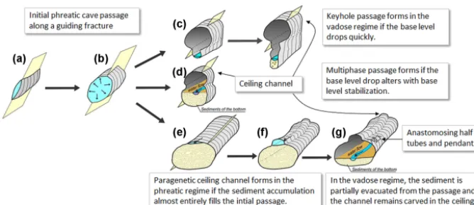
colour-Figure 1. Schematic evolution of the passages in phreatic and vadose hydrological regime under conditions of high sediment flux and following abandonment (modified after Farrant and Smart, 2011). Further description of the stages is Sect. 2.1.

ing. However, more information can be inferred if the point representation is converted into a continuous digital surface model. Afterwards, sophisticated methods for analysing the Earth surface morphology can be applied, which is the main domain of geomorphometry. Traditionally, a bivariate func-tion has been sufficient to analyse the ground surface (Mi-tas and Mi(Mi-tasova, 1999). Digital elevation models (DEM) are usual representations of the Earth surface for which the methodological concept of digital terrain analysis is well de-veloped and a plethora of geomorphometric tools exist in various kinds of software (Hengl and Reuter, 2009). In geo-sciences, 2-D arrays are the most popular representation of DEMs among the users. The main reason is due to the ease of manipulation and design of algorithms. However, the ap-proach reaches its limitations for geomorphometry of 3-D volumetric surfaces such as caves (Roncat et al., 2011; Gal-lay et al., 2015b).

The aim of this paper is to present a novel methodology of deriving morphology information for the identification of ceiling channels using a high-resolution digital cave surface model and geomorphometric analysis. The high level of de-tail captured by TLS coupled with new 3-D modelling tools enable us to study specific cave landforms with unprece-dented accuracy. This paper presents new aspects of studying cave genesis facilitating the traditional 2-D geomorphomet-ric tools and innovative 3-D methods of computer graphics. The methodology is demonstrated with the data acquired by TLS in the Domica cave, Slovakia, in 2014 (Gallay et al., 2015a). This paper also provides new evidence of the hydro-logical regime acting during the cave formation.

2 Research background

2.1 Evolution of ceiling channels

Ceiling channels originate as a result of erosional action and corrosion of underground water flow, but they can evolve

un-der various hydrological regimes (Ford and Williams, 2007; Pasini, 2009; Farrant and Smart, 2011). Most often there is initially a phreatic tube, which has formed along a guid-ing fracture in the rock (Fig. 1a). The phreatic tube grows in all directions (Fig. 1b). In case the seepage drops down, the phreatic regime changes to the vadose regime. The wa-ter stream is further incising the rock downwards. If the base level drops quickly, a keyhole passage is formed by the sub-sequent downward incision of the stream (Fig. 1c). The ini-tial tube is abandoned and remaining as a half tube carved in the cave ceiling. Typically, the initial guiding fracture can be observed in the ceiling. A multi-phase evolution passage is formed if phases of base level drop and base stabilization alter (Fig. 1d).

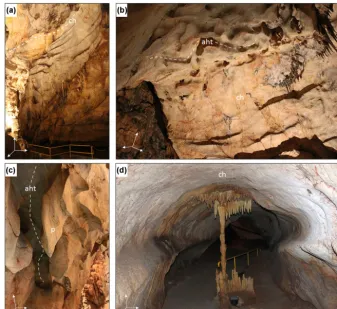
Figure 2. Examples of ceiling channels (ch), pendants (p), and anastomosing half tubes (aht) in the Domica cave as speleoforms associated with the phreatic regime. Presence of the speleoforms in the ceiling and walls of the Gothic Dome indicate paragenetic (antigravitational) development (a, b, c), while it is more difficult to infer from the “dry passage” (Suchá chodba in Slovak) (d) from where much of the accumulated sediment was not evacuated and the passage was reshaped during multiple phases of vadose and phreatic conditions. The highest parts of the channels can be situated as high as 16 m (a, b) or 2 m above the floor on sediment accumulation (d).

sediments can be found near the ceiling vault as the evidence of the former accumulation fill.

First explanation of such formation of cave passages is at-tributed to Renault (1968), who termed the process as para-genesis. However, 3 decades earlier, Roth (1937) identified ceiling channels and explained their morphogenesis in the same way in his study on the evolution of the Domica cave in the former Czechoslovakia. Roth (1937) was published in Czech with a French summary, which limited its wider readership (Bella and Bosák, 2015). Pasini (2009) provided a detailed reasoning of the paragenetic formation of ceiling channels and suggest the more appropriate term “antigrav-itative erosion”. Paragenesis is well-known and widespread in gypsum and limestone caves. Favourable environmental conditions for antigravitative erosion typically occur in the contact karst settings where there is sufficient sediment in-put into caves. Most sediment enters cave systems via stream sinks. Large, low gradient river caves are often subject to par-agenetic development (Farrant and Smart, 2011). The sedi-ment influx may be semi-continuous, with paragenesis oc-curring throughout the cave’s development. The Domica–

Baradla cave system is an example when allogenic drainage led to significant alluviation and paragenetic development (Bosák et al., 2004). The system evolved in the edge of a limestone block, which is in contact with gravel–clay delta-like sediments. Paragenesis is often thought to be of local in-terest, but increasing observations seem to indicate that many caves could be partially, if not almost completely, formed by this process (De Waele et al., 2009). Mapping the morphol-ogy of the cave ceiling thus provides essential evidence of the cave system formation. However, the morphological in-dicators are varying in size and abundance and they are often difficult to reach for humans. Therefore, recently emerging high-resolution mapping technologies, such as laser scan-ning, have potential to overcome the obstacles.

2.2 Benefits of terrestrial laser scanning and geomorphometry in cave mapping

mapping in the last decade (Canevese et al., 2009; Rüther et al., 2009; Buchroithner et al., 2011; Zlot and Bosse, 2014; Gallay et al., 2015a; Idrees and Pradhan, 2016). The scanner emits laser beams and records the reflected electromagnetic energy with a high frequency and accuracy. This generates a point cloud withx,y,zcoordinates providing a very de-tailed 3-D record of the cave morphology (of the order of millimetres), which can be used for visualization, profiling, and measurements (Buchroithner, 2015). The points can be used for generation of 3-D cave surface models, which brings the possibility of detailed geometric analysis of the cave mor-phology.

Geomorphometry has traditionally been used in geomet-ric analysis of terrain (land surface) (Evans, 1972; Krcho, 1973; Pike et al., 2009; Minár et al., 2013). Many morpho-metric parameters indicate likely occurrence of geomorpho-logical processes, such as water erosion, landslides, or flood-ing (Hengl and MacMillan, 2009). However, specific forms such as caves or overhangs represent 3-D objects which re-quire a more complex approach including new, 3-D mod-elling methods and tools.Traditional approximation of ter-rain surface with a bivariate functionz=f (x,y)is limited for 3-D surfaces as there is more than one value of altitude z for a given location (x, y). Nevertheless, the bivariate ap-proach can also be applied for modelling parts of the cave system, for example, cave ceiling or cave bottom. McFar-lane et al. (2015) used this idea in identification of swiflets’ nests in the Bomatong cave by extracting the upper part of the cave from a TLS data set and modelling the ceiling as a raster DEM. Another solution is to transform the orienta-tion of the modelled TLS point cloud so that it satisfies the condition of unambiguity of the bivariate function. Starek et al. (2013) used the approach to model the lateral river bank erosion. Mahmud et al. (2015, 2016) worked with the dis-tance from the scanner instead of the altitude to identify in-filtration properties in limestone by the means of 2-D mor-phological analysis of the Golghota cave ceiling, Western Australia. However, it should be emphasized that generat-ing the 2-D raster-DEM-like representations of the cave sur-face is possible only from a high-resolution 3-D point cloud representation of the cave acquired via laser scanning. Data surveyed by traditional cave mapping methods are not suffi-ciently detailed to be used in such a 2-D geomorphometric analysis.

The bivariate approach can be extended to a trivariate anal-ysis of 3-D phenomena, where the scalar parameter w is modelled as w=f (x, y, z) (Hofierka and Zlocha, 1993). This concept is applicable for phenomena distributed in a 3-D space (e.g. air temperature, air pressure, water infiltration rate) and it is implemented in the geographic information system GRASS (Petras et al., 2015). However, the concept cannot be applied to 3-D landforms as the Earth surface is a 2-D boundary interface existing in a 3-D spatial domain. One of the solutions applicable for digital 3-D Earth surface mod-elling is to use polyhedral meshes (meshes). Polyhedral 3-D

meshes are vector-based representations commonly used in computer graphics. Such a mesh is generated by connecting input 3-D points into a polyhedral network. Most often trian-gular facets are used which is similar to modelling the terrain with a triangulated irregular networks (TINs).

Currently, 3-D cave surfaces from laser scanning data need to be generated using other kinds of software, which have been recently developed in relation to the rapidly emerging 3-D data acquisition methods, for example, Blender, Meshlab, Polyworks, CloudCompare, 3-DReshaper, Geomagic Studio, VMTK. Primarily, the main application of the software is in modelling surfaces of objects other than the Earth’s surface mainly for cultural heritage science, archaeology, architec-tural design, medicine, forensics, and civil engineering. This kind of software emerged in times of multiple-core process-ing units with a 64 bit architecture. Therefore, the algorith-mic design is made to exploit parallel processing for fast computation and rendering of massive 3-D data sets even on a laptop. However, the tools can be applied to 3-D point clouds representing geographic landscapes. As the software is not specifically oriented to the analysis of cave morphol-ogy, specialized tools have to be used. For more details on methodologies for this issue, the reader is advised to consult works by Roncat et al. (2011), Jaillet et al. (2013), Cosso et al. (2014), Hoffmeister et al. (2015), Silvestre et al. (2015), or Gallay et al. (2015a, b), which exploited commercial soft-ware and open-source softsoft-ware for 3-D cave surface mod-elling. In this manner, the new software tools fill the gap which has emerged when the traditional 2-D geomorphome-tric approach adopted in GIS hit its limitations in handling 3-D surfaces. Various tools have been implemented for this task within the GIS platform, e.g. 3-D analyst in ArcGIS (ESRI, 2015) or r3.modules in GRASS GIS (Neteler and Mitasova, 2008; Neteler et al., 2012), but still further research is needed to implement new 3-D analytical tools and to enable faster data rendering and processing.

3 Study site

Nat-Figure 3. Location of the scanned part of the Domica cave with orthogonal projection of the Domica–Baradla cave system according to Droppa (1972).

ural Heritage Site since 1997. Panorama photography views of selected parts of Domica are available as a virtual tour on http://www.panoramika.sk/firma/jaskyna-domica/10056/. Laser scanning of the cave provided non-disturbing means for highly detailed 3-D parameterization of the cave corridors enabling to study its morphology and acting as a catalyst for further research and educational initiatives.

Domica is a typical example of a fluviokarst cave, which was formed by several underground water streams in lime-stones. The cave was formed by corrosive-erosive processes caused by superficial fluvial water and temporary streams, which sank underground at the contact of the Middle Triassic white limestones and the Pontian fluvial–lacustrine gravel– sand–clay sediments (Bella, 2001). The tectonic framework was generated by south to southeast oriented pressures, which caused stress, and the compression was realized in the range of directions of north–south to northwest–southeast (Gaál and Vlˇcek, 2011). Bella et al. (2014) performed cos-mogenic nuclide dating of quartz pebbles cemented in the upper parts of Domica (340 m a.s.l.). Their results suggest that the upper level (338–340 m a.s.l.) began to form after uplifting the region above sea level earlier than the Middle Pliocene (3.47±0.78 million years) when the current hydro-graphic network was being established. The middle level is located 10–12 m below the uppermost level. The lowest

evo-lution level of Domica was found at one place by drilling at 318 m a.s.l. (Droppa, 1972).

The cave is a result of the underground flow of Styx and Domický potok shown by the oval shapes of the corridors and the quantity of allochtone pebbles found in the system. Both water streams are strongly influenced by the amount of atmo-spheric rainfall, which was observed according to the hydro-logical monitoring of water discharge of Styx and Domický potok inside the cave and simultaneously monitoring precipi-tation outside the cave during 1999–2001 (Peško, 2003). Av-erage annual air temperature in the cave varies between 10– 11◦C and air humidity is around 95–98 %. The average an-nual outdoor air temperature is between 8 and 8.3◦C and the mean annual precipitation varies around 635 mm based on monitoring during 1955–2004 at the closest meteorological station in Plešivec, 10 km north of Domica (Haviarová and Gruber, 2005). The water discharge of Styx and Domický po-tok is normally very low (0.4–0.5 L per second), however, it quickly increases during rapid rainfall or snow thaw when the soil is saturated or frozen. In the recent past, several rainfall events caused major flooding in the cave. This flooding was also due to inappropriate agricultural practise (Bella, 2001; Gaalova et al., 2014).

their sedimentary load in the cave what resulted in upward erosional incision of the stream, thus the formation of ceil-ing channels (Bella, 2000). The channels were first described by Roth (1937), who published an extraordinary study on the morphogenesis of the cave reconstructing its palaeohy-drography (Bella and Bosák, 2015). His work was further extended by other followers (e.g. Kunský, 1950; Droppa, 1972), who mapped the cave and measured physically ac-cessible parts of the cave. The last complex surveying was done by the Geological Survey, national enterprise, Spišská Nová Ves in 1975 (Novoveský, 1975). However, the maps portray only the cave bottom not the ceiling. In places where the height of cave corridors restrains closer study of the ceil-ing, the geometric properties of channels were just estimated. In particular, the high ceiling could be only partially observed for obstacles or properly measured. The uniqueness of the Domica cave and the interest of wider research community in this area were the main driving factors to acquire a highly detailed 3-D representation of this underground landscape.

4 Data and methods

4.1 Terrestrial laser scanning

The data used in the presented research were acquired with a terrestrial laser scanner in combination with differential satellite positioning using real time kinematic method (RTK-GNSS) surveying within a 5-day mission in March 2014 in the Domica cave, Slovakia. Although the cave is drained by the permanent subsurface water flow Styx, the water level was very low and the cave was generally dry. This provided favourable conditions for scanning with an infrared laser. The survey is thoroughly described and compared with other sim-ilar surveys in Gallay et al. (2015a); hence we describe only the main facts. FARO Focus 3-D scanner was used to scan around 1600 m of the cave from 327 individual scanning po-sitions within 40 h in total. The majority of individual scans were acquired at a scanning resolution given by point spac-ing of 7.6 or 6.1 mm at the range 10 m away from the scanner, respectively. In some instances the scanner was set to 3 mm spacing of measured points at 10 m range especially in large caverns with high ceilings. The final point cloud contained over 11.9 billion of measured points representing the entire show cave and some parts inaccessible by public. The total area of the scanned cave footprint was about 15 000 m2.

Semi-automatic registration of the individual scans was carried out using reference spheres placed in each scene and this method achieved an overall registration error of 2.24 mm (root-mean-square error, RMSE). Three RTK-GPS points surveyed outside the cave visitor centre and one point from older cave survey (Novoveský, 1975) in the rear north part of the cave were used to transform the final registered point cloud from its local coordinate system to the Slovak national cartographic system (S-JTSK) with the vertical

ref-erence to the Baltic Datum after adjustment using the local geoid model. The transformation achieved the total accuracy of 21 mm (RMSE). The registration of scans and georefer-encing was conducted in the SCENE8 software by FARO. The SCENE data project is used to manipulate the point data in the full spatial extent and full resolution. For other ana-lytical tasks and 3-D modelling, the points are exported into the PXT format which is an ASCII based interchange format for point cloud data used by the Leica Cyclone software. The format stores normal vectors for each point oriented with re-spect to the scanning position from which the point had been located. The point cloud provides a very high detail of the order of few millimetres, which enables viewing even small geomorphological features such as soda-straw speleothems.

4.2 Generating a 3-D cave surface model

It is not convenient and efficient to analyse the entire georef-erenced point cloud at the highest level of detail (full resolu-tion). Either parts of it are selected and the selected points are further used for meshing or other analysis in full resolution or the original cloud is decimated to model the cave surface at lower resolutions. Despite some loss of information, the decimation (i.e. subsampling) homogenizes spatial distribu-tion of the points into a semi-regular spacing thus provid-ing control of the level of detail (spatial scale). First, for a more convenient handling, the original points were exported from the SCENE project into the PTX format by sampling every 7th point in horizontal and vertical direction with re-spect to their origin (i.e. scanner position). This procedure reduced the number of the exported points to almost 2 %. However, it was still sufficient to keep the level of detail required for the analysis presented in this paper (Fig. 4a). Afterwards, the cloud was subsampled in the open-source CloudCompare software (Girardeau-Montaut, 2006, 2015). Two data sets were derived by subsampling with the crite-rion of minimal distance between two points. This means that the points are not closer to each other than the speci-fied value. The points were reduced having a minimal spac-ing of 1 and 5 cm, respectively (Fig. 4b). Before further use, the clouds were manually cleaned in Meshlab (Cignoni et al., 2008; Cignoni and Ranzuglia, 2014) from noise and out-liers which originated mainly due to the presence of water. The new clouds were further used in the analysis of the cave surface morphometry based on 2-D raster representation of digital elevation models and 3-D meshes (Fig. 4c).

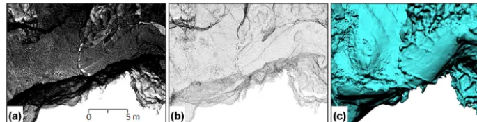
Figure 4. Point cloud from the Gothic Dome orthogonally projected on a horizontal plane representing 2 % of the full resolution as exported from the SCENE project (a), after subsampling the points at 5 cm minimal spacing (b), and as a continuous 3-D cave surface model (c) generated from (b) with the octree depth of 12.

2006). For 3-D modelling of the Domica cave, we adopted a triangular 3-D-mesh consisting of triangular facets. Each facet is defined by a set of three vertices and its orientation (the angle of azimuth and slope) is defined by a vector nor-mal to the facet. Usually, it is meaningful to reduce the in-put point cloud before these steps are performed to test the methodological approach.

The Meshlab software (Cignoni and Ranzuglia, 2014) was used to generate a 3-D triangular mesh from the input point clouds. Meshlab is free and open-source software for mesh processing and editing capable of working with numerous 3-D file formats. Generation of a 3-3-D surface model requires that points are assigned with normal vectors. In our case, the points had normals assigned during scanning with respect to the scanner position. Otherwise, it would be necessary to calculate the normals for which several algorithms exist in the software. The surface model (mesh) can be reconstructed using several algorithms. We tested the Poisson surface re-construction approach by Khazdan et al. (2006). Silvestre et al. (2015) used this procedure to model the surface of a cave chamber and identified stalactites based on local minima of the 3-D surface. The Poisson reconstruction of the 3-D sur-face is based on the observation that the normal field of the boundary of a solid can be interpreted as the gradient of the solid’s indicator function. Therefore, given a set of oriented points sampling the boundary of a solid, a 3-D-mesh can be obtained by transforming the oriented point samples into a continuous vector field in 3-D. This is performed finding a scalar function, whose gradients best match the vector field, and extracting the appropriate isosurface. A thorough defi-nition of the Poisson surface reconstruction can be found in Khazdan et al. (2006). The approach is also implemented in CloudCompare. It is important to mention that the vertices of the reconstructed triangular 3-D meshes do not coincide with the points of the survey points as it is in the case of the Delaunay triangulation. With this algorithm, octree depth is the key input parameter controlling the level of surface de-tail. It is the maximum depth of the octree hierarchy that is used for surface reconstruction by fitting an indicator func-tion modelling the 3-D surface. The method adapts the octree to the sampling density, therefore the specified

reconstruc-tion depth is only an upper bound. The number of vertices (also facets) comprised in the resulting 3-D mesh increases with the increasing value of the octree depth. After recon-structing the 3-D mesh, further processing and surface anal-ysis was performed, such as removing non-manifold edges, duplicated vertices, decimation of the mesh, or the mesh pa-rameterization.

The 3-D model for the full spatial extent of the scanned cave passages was generated using the Poisson surface re-construction algorithm with the octree depth setting of 12. The data sets used originated from subsampling the origi-nal point cloud at 5 cm minimal spacing of points. The re-sulting model contained 4.77 million of vertices and it was stored in the binary Stanford polygon file format (PLY) hav-ing 349 MB (Fig. 4c). Selected parts of the cave were mod-elled in higher detail from the point cloud decimated to 1 cm minimal spacing of points and with the octree depth of 14.

4.3 Identification of ceiling channels using 2-D geomorphometry

Caves are subsurface landforms with a complex morphology. Despite the cave being a true 3-D landform, it can be partially modelled and analysed with traditional 2-D geomorphome-try. The geomorphometric tools usually applied for 2-D grid-ded elevation data can be used to identify and measure par-ticular features associated with the speleohydrological pro-cesses. For example, the 3-D point cloud can be filtered in order to extract the points of the highest elevation represent-ing the cave ceilrepresent-ing. In the next step, DEM of the cave ceil-ing can be generated from the points. Similarly, points of the lowest elevation can be extracted to generate DEM of the cave bottom part.

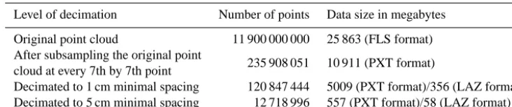
Table 1. Summary of point cloud reduction.

Level of decimation Number of points Data size in megabytes

Original point cloud 11 900 000 000 25 863 (FLS format)

After subsampling the original point

235 908 051 10 911 (PXT format)

cloud at every 7th by 7th point

Decimated to 1 cm minimal spacing 120 847 444 5009 (PXT format)/356 (LAZ format)

Decimated to 5 cm minimal spacing 12 718 996 557 (PXT format)/58 (LAZ format)

compressed version of the LAS which is a public file for-mat for the interchange of 3-D point cloud data data between data users defined by (ASPRS, 2014) format. In this way the storage demand decreases (Table 1) and the point cloud can be processed very efficiently in LAStools (Isenburg, 2014). We used the open-source unlicensed lasgrid utility to gener-ate the raster DEM of cave ceiling by extracting the high-est altitude value of a point within a squared grid cell of 25 cm size. Similarly, the lowest altitude value of a point was extracted to generate the raster DEM of cave bottom. The decimated point clouds of 5 cm spacing were used for this purpose. The DEMs represent the orthogonal projection of the cave morphology on a horizontal plane. The DEMs were imported into a GRASS GIS geodatabase (Neteler and Mitasova, 2008) where they were further handled by tools dedicated for raster data analysis. Relative height differences between the ceiling and the above-surface were calculated using a digital elevation model of terrain (DTM) generated from an airborne laser scanning (ALS) data set. The data originated during a mission flown in August 2014 by Pho-tomap s.r.o., Košice over a wider area of the Domica cave. The accuracy of measurement in open areas is reported at 0.1 m of 1σby the data supplier. The density of laser returns classified as ground points varied between 0.5–8 points per m2which allowed for production of high-resolution gridded DTM of 1 m cell size. The workflow of processing the ALS data is more specifically described in Hofierka et al. (2016). Tables 2 and 3 summarize the generated data and key param-eters of the commands used.

The ceiling channels can be perceived as ridges of the cave closed volume. The algorithm used for calculating the ceiling line is based on the modified approach of Hardin et al. (2012), who extracted sand dune ridgelines. Their method is based on least cost path algorithm and traces the DEM cells of the highest elevation value between two points. We used a normalized ceiling height (DEM_CH_NORM) before calculating the cost surface model as the altitude values in our case are higher numbers (hundreds of metres) as opposed to the coastal dunes. By this means, we avoided calculation of very small cost values approaching zero which reach the limitation of the software at a certain level of decimal pre-cision. As a result, the approach can be universally used in other kinds of landscape. The constant of 300 improves de-lineation of the line; however, the value can be changed

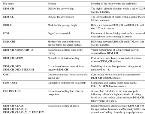
Table 2. Summary of raster data derived from 3-D point cloud in LAStools and GRASS GIS.

File name Purpose Meaning of the raster values and their units

DEM_CH DEM of the cave ceiling The highest altitude of points within a cell of 0.25 by 0.25 m, in metres.

DEM_CL DEM of the cave bottom The lowest altitude of points within a cell of 0.25 by 0.25 m, in metres.

DOD_C Model of the passage height Difference between DEM_CH and DEM_CL, cell size 0.25 m, in metres.

DTM Digital terrain model Elevations of the surficial ground surface measured with airborne laser scanning, in metres.

DOD_CHT Model of the depth of the cave Difference between DEM_CH and DTM, cell size ceiling below the terrain surface 0.25 m, in metres.

DEM_CH_CONTOURS_05 Extraction of contour lines of the Vector contour lines of 0.5 m vertical interval

ceiling extracted from DEM_CH.

DEM_CH_NORM Normalized altitude of ceiling Cost surface raster based on normalized altitude values of DEM_CH, unitless.

DEM_CH_NEG, Extraction of stream network from Modelling of water flow paths on ceiling model DEM_CH_NEG_STREAMS negative DEM_CH multiplied by−1.

COST Cost surface model for extraction of a Cost surface raster calculated as exponential of

ceiling line DEM_CH_NORM, unitless.

CUM_COST Cumulative cost between two points Cumulative cost surface raster based on the COST_SURFACE raster, unitless.

CEILING_LINE Extraction of ceiling line between A raster line calculated as the least cost path two points following cells of the highest altitude of ceiling,

based on a cost surface calculated from DEM_CH, binary values of 0 and 1.

DEM_CH_CLASS, Extraction of ceiling channels Geomorphometric classification of DEM_CH with

DEM_CH_CLASS_23, the approach of Jasiewicz and Stepinsky (2013) and

DEM_CH_CLASS_23_CLUMP_ELV, extraction of ceiling channels by map algebra and

DEM_CLASS_CC Boolean logic.

4.4 Analysing the cave surface using 3-D geomorphometry

The generated cave surface 3-D model enabled a new range of analysis parameterizing the cave morphology more accu-rately and from different perspective than with the DEM ap-proach. The analysis was performed in Meshlab and Cloud-Compare where the suite of tools for analysing 3-D geome-try is very diverse and customable. Volume and surface area were calculated for meshes generated with differing octree depths with the compute geometric measures filter in Mesh-lab. From the visualization point of view, just the sole view-ing of the generated 3-D cave surface model is a useful means of inspecting the cave morphology in searching for ceiling channels and associated forms. Changing the light source an-gle reveals particular morphological features. However, more powerful measures than interactive shadowing can be calcu-lated to improve perception of the 3-D shape and to help identifying the features. We explored various 3-D surface

quality measures such as altitude, ambient occlusion and cur-vature parameters to colourizing the 3-D mesh based on the calculated parameter values.

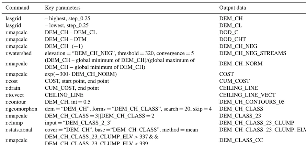
Table 3. Computer commands and their key parameters for generating the data listed in Table 2.

Command Key parameters Output data

lasgrid – highest, step_0.25 DEM_CH

lasgrid – lowest, step_0.25 DEM_CL

r.mapcalc DEM_CH – DEM_CL DOD_C

r.mapcalc DEM_CH – DTM DOD_CHT

r.mapcalc DEM_CH·(−1) DEM_CH_NEG

r.watershed elevation=“DEM_CH_NEG”, threshold=320, convergence=5 DEM_CH_NEG_STREAMS

r.mapcalc (DEM_CH – global minimum of DEM_CH)/(global maximum of DEM_CH_NORM

DEM_CH−global minimum of DEM_CH)

r.mapcalc exp(−300·DEM_CH_NORM) COST

r.cost COST, start point, end point CUM_COST

r.drain CUM_COST, end point CEILING_LINE

r.to.vect CEILING_LINE CEILING_LINE_VECT

r.contour DEM_CH, int=0.5 DEM_CH_CONTOURS_05

r.geomorphon dem=“DEM_CH”, forms=“DEM_CH_CLASS”, search=20, skip=4 DEM_CH_CLASS

r.mapcalc DEM_CH_CLASS=3||DEM_CH_CLASS=2 DEM_CLASS_23

r.clump input=“DEM_CLASS_2_3” DEM_CH_CLASS_23_CLUMP

r.stats.zonal cover=“DEM_CH”, base=“DEM_CH_CLASS”, method=mean DEM_CH_CLASS_23_CLUMP_ELV

r.mapcalc DEM_CH_CLASS_23_CLUMP_ELV>337 & & DEM_CLASS_CC

DEM_CH_CLASS_23_CLUMP_ELV<339

Curvature of a surface is a significant parameter com-monly calculated in DEM analysis. In the presented study, we explored the multi-scale 3-D cave surface curvature pa-rameterization with the filter for colorizing curvature of an algebraic point set surface (APSS) by Guennebaud and Gross (2007) filter in Meshlab. Gallay et al. (2015b) tested calcula-tion of mean surface curvature at various levels of scale for a small section of the Domica cave. Their approach uses a lo-cal moving least-squares (MLS) fitting of algebraic spheres with intuitive parameters for curvature control of the fitted spheres. Computation of the curvatures requires points, mesh vertices, or facets equipped with oriented normal. The spatial scale of the fitted sphere can be controlled by setting the MLS filter scale, which is a value relative to the local point spacing of the vertices. The higher is the filter scale value the larger is the neighbourhood of the vertex for which the sphere is fitted and the curvature is calculated. The curvature value repre-sents the inverted radius of the sphere tangent to the points in the defined neighbourhood of a vertex. We calculated the principal curvatures K1 and K2, mean curvature, and Gauss curvature. K1 curvature parameterizes the minimal curvature of the surface while K2 curvature defines the maximal cur-vature of the surface (Willmore, 2012). Gauss curcur-vature is the product of K1 and K2 curvatures. The average of K1 and K2 values for a given vertex is the measure of the overall sur-face convexity/concavity, i.e. mean curvature parameter. As a result, generally convex features, such as stalactites, sta-lagmites, or pendants, have positive mean curvature values while concave features, such as sinks, cavities, half tubes, or sinks have negative values. Lai et al. (2014) used the

curva-ture of a 3-D mesh as a measure of the surface roughness of rock faces.

Roughness of the 3-D cave mesh was parameterized with the roughness tool implemented in CloudCompare. For each point, the “roughness” value is equal to the distance between this point (mesh vertex) and the best-fitting plane computed on its nearest neighbours. The size of spatial scale is con-trolled by the kernel radius parameter, which is the radius of a sphere centred on each vertex. We tested several radius settings and finally used the radius of 0.5 and 5 m, which ac-curately depicted the anastomosing half tubes and the ceiling channels, respectively.

5 Results and discussion

han-dle the data. Therefore, we generated a tool for interactive visualization and simple analysis of the generated data via the Web interface, which is presented in Sect. 5.3.

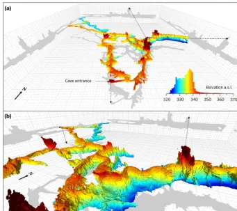
The 3-D point cloud acquired by TLS is the key data source, which enabled exact quantification of the cave ceiling and from which we derived 2-D and 3-D models represent-ing the cave surface. To familiarize the reader with the overall layout of the analysed Domica cave system, Fig. 5 provides perspective view of the 3-D cave surface model with its or-thogonal projections. The presence of the ceiling channels can be clearly observed in the detail view as the elongated and horizontally winding half tubes in the cave roof. Also, we emphasize the fact that the top parts of the channels formed in horizontal levels, which, in some places, are disrupted by younger vertical or subvertical forms, such as chimneys, re-lated to tectonics.

5.1 Cave ceiling analysis based on 2-D geomorphometry

5.1.1 DEM-based analysis

The ceiling of Domica was modelled by a bivariate approach, which allowed for using diverse geomorphometric methods developed for 2-D digital terrain analysis with DEMs. The generated DEM data sets and DEM-derived data represented the cave ceiling morphology orthogonally projected on a horizontal plane (Figs. 6 and 7). Table 4 presents summary statistics of the gridded elevation models. The statistics are valid for the scanned part of the cave.

The footprint area of the cave based on DEMs is 1934 m2. The altitudes of the scanned cave system range between 322.51 m (minimum of DEM_CL) to 368.58 m (maximum of DEM_CH). The ceiling altitude ranges within 46 m but its height is influenced by the presence of speleothems or chim-neys. Therefore, quantile values are more informative in as-sessing the ceiling altitude. Majority of the ceiling evolved within 328.92 to 339.93 m. However, two peaks of the sta-tistical distribution can be observed in the histogram of the ceiling highest elevation (Fig. 6a). The lower maximum re-lates to the youngest evolution level of the Virgin passage developed at about 329 m a.s.l. (segment A in Fig. 8). The higher maximum is associated with the ceiling of the older evolution stages (segments B–F in Fig. 8) at about 338.75– 340 m. The highest 10 % of the ceiling above 340 m is related to the concave features that originated as a result of younger ceiling collapse along tectonic fractures, which is well seen in side projections of the 3-D model in Fig. 5.

The extraction of the highest and lowest points of the orig-inal point cloud enabled calculation of a digital model of difference (DOD_C) as the relative ceiling height above the cave floor (Table 4). The morphology of the cave bottom (DEM_CL) is influenced by human interference when build-ing infrastructure for the show cave, but the statistics provide useful data for comparison (Fig. 6b). The DOD_C model is

more revealing as it quantifies the openness of the cave in-terior and the amount of the eroded material (Fig. 6c). The range of the heights for a certain location is 32.42 m and at 90 % of locations the cave ceiling less than 10 metres high.

The scanned cave passages have developed relatively deep below the terrain surface (Fig. 6d). Despite that, there are some chimneys almost 30 m tall, 90 % of the ceiling is more than 34 metres and 75 % more than 59 m below the terrain, respectively (DOD_CHT). No marked signs of the ceiling collapses on the above surface can be observed on the lidar-based DTM (Fig. 2). There are dolines north of the known cave passages but no connection has been proven yet.

5.1.2 Least cost path analysis

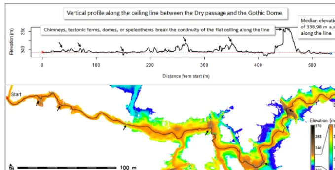
The cave 3-D model (Fig. 5) and the ceiling DEM (Fig. 6a) clearly reveal winding forms in the highest parts of the ceil-ing not notceil-ing the chimneys or stalactites. These are the ceiling channels, which are most markedly developed in the Dome of Mysteries, the Majko’s Dome, and the Gothic Dome. The channels thus form ridges in the DEM_CH for which a ridgeline, i.e. ceiling line, was automatically ex-tracted. Considering the ceiling morphology, we divided the ceiling into six contiguous segments marked A–F in Fig. 7 for which elevation, length, and sinuosity statistics were cal-culated (Table 5). Figure 8 shows the ceiling line and its lon-gitudinal profile between the “dry passage” (Suchá chodba in Slovak) and Gothic Dome (segments B–D in Fig. 7). It can be seen that the profile is not smooth or flat as it would be expected in case of a generic river profile. The reason is that, besides the downwards flow of water, the formation of ceil-ing could be influenced by hydraulic pressure in the phreatic regime and paragenesis. After the water level decreased, and the conditions changed to vadose or epiphreatic, speleothems developed or the ceiling collapsed resulting in formation of chimneys. The ceiling line thus follows the DEM cells of the highest altitude. Nevertheless, the ceiling line very well indi-cates the presence of the ceiling channels. The longitudinal profile shows most of the parts preserved as horizontal lev-els. Interestingly in these flat parts, no obvious inclination of the profile line with respect to the flow direction can be identified. The same stands for other ceiling segments. The interruptions of the profile act as statistical outliers; there-fore, quantiles are most appropriate to infer the trends in the elevation of the derived ceiling lines.

Figure 5. 3-D model of the Domica cave oriented towards the north (a) and its detailed view towards north-west (b) showing a meandering ceiling channel. The model is coloured by the value of altitude above mean sea level which distribution is shown by the histogram. The 3-D geometry is orthogonally projected on the XY, YZ, and XZ planes. The size of the major and minor cells in the background grid is 20 and 5 m along all three axes, respectively. Note the flat, horizontal ceiling levels projected on the vertical XZ and YZ planes.

Table 4. Summary statistics of the DEM data sets parameterizing morphology the scanned part of the Domica cave.

DEM Cell Min Max Range Mean SD 1st quart. Median 3rd quart 10th perc. 90th perc.

data set count [m] [m] [m] [m] [m] [m] [m] [m] [m] [m]

DEM_CH 221,772 322.51 368.58 46.07 335.49 4.79 331.37 336.69 338.75 328.92 339.93

DEM_CL 243,216 318.99 349.34 30.35 330.93 4.62 326.72 331.16 334.91 324.85 336.72

DOD_C 221,772 0.00 32.42 32.42 4.26 3.99 1.48 3.151 5.79 0.26 9.97

DOD_CHT 221,772 −99.79 0 99.79 −68.23 20.63 −82.636 −72.97 −59.54 −90.53 −34.26

of the Domický potok river. Their median elevation is sim-ilar (339.78 and 339.95 m) and also it is the highest among the three groups. In comparison with the segment A, the seg-ments B–F are mutually more similar and represent the same evolution phase. These fact were speculated in previous stud-ies (Roth, 1937; Kunský, 1950; Droppa, 1972; Bella, 2000) but our approach provided exact measurement and evidence. Moreover, the level of meandering was quantified by the sinuosity index SI (Table 5). According to the conventional classes of the index, the ceiling lines are not straight, most of them are twisty which, however, cannot by attributed only to lateral meandering, but tectonics also affects the ceiling line. The most markedly meandering ceiling line is the D

seg-ment, which has a nice marked meandering half tube chan-nel. The meander wavelength gradually shrinks from 30 m in the Dome of Mysteries to 15 m in the Gothic Dome.

5.1.3 Ceiling surface classification

col-Figure 6. Raster based models with histograms representing the highest cave ceiling altitude (a), lowest altitude (b), vertical difference

between the cave bottom and ceiling (c), and the ceiling depth below the terrain surface (d). The histogramyaxis represents the number of

raster cells in hundreds.

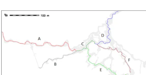
Table 5. Summary of elevation and length statistics of the ceiling line segments as shown in Fig. 8.

Cave Min Max Range Mean SD Q₂₅ Median Q₇₅ IQR Length Straight SI∗ SI class segments [m] [m] [m] [m] [m] [m] [m] [m] [m] [m] length

[m]

A 327.06 338.90 11.83 330.48 1.48 329.58 329.98 331.15 1.57 356.28 261.00 1.37 twisty B 336.90 340.67 3.76 338.92 0.45 338.67 338.77 339.08 0.41 164.71 140.00 1.18 winding C 338.57 344.73 6.16 339.56 1.19 338.90 339.02 339.65 0.75 95.41 67.00 1.42 twisty D 335.99 351.72 15.73 339.31 2.19 338.39 338.87 339.14 0.75 225.35 135.00 1.67 meandering E 334.80 351.98 17.18 340.09 1.69 338.99 339.78 340.71 1.72 235.05 162.00 1.45 twisty F 337.84 368.91 31.07 341.30 5.04 339.46 339.95 340.56 1.1 203.08 147.00 1.38 twisty A–F 328.74 368.91 40.17 337.48 5.09 332.42 338.88 339.84 7.42 1279.88 NA∗ NA NA

∗_{SI – sinousity index; NA – not applicable.}

Figure 7. Segments of ceiling lines with assigned letters as refer-enced in the text and as reported in Table 5.

lapses, and formation of speleothems. Their surface is

hor-Figure 8. Longitudinal profile along the automatically delineated ceiling line of overlaid on top of the raster DEM_CH.

Figure 9. Classification of the ceiling surface (DEM_CH) of the Majko’s Dome and the Gothic Dome (Fig. 3) in GRASS GIS to extract the ceiling channels as landforms. Ceiling channels are classified with the r.geomorphons module as ridges and some parts as summits (a). The two categories are extracted as binary rasters with r.mapcalc and small clusters are removed with r.neighbors (b). The areas are clumped into individual spatial units for which elevation summary statistics were calculated. Median elevation (c) most appropriately separated the ceiling channels from other ridges and summits (d).

izontal continuity of the channels (Fig. 10b). For example, the sequence of the channels 14, 19, 21 suggests common formation by the same palaeostream in the same time but the median of the channels 15 and 20 is 40–50 cm lower than the median of channel 22. Contiguity of the channels is disrupted by a tall chimney, which is horizontally perpendicular to the ceiling line and spans up vertically about 30 m. Similar cases exist in other parts of the cave (e.g. segments 21, 17, 16). They have been discussed since 1930s; however, no means for exact quantification were available until the emergence of high-resolution laser scanning and 3-D-modelling.

5.2 Cave ceiling analysis based on 3-D geomorphometry

Figure 10. Ceiling channels resulting from the semi-automatic classification of the Domica ceiling, which were grouped according to their median elevation (a) reported in Table 6 and interpretation of their vertical displacement (b).

Table 6. Ceiling channels identified in the DEM_CH classification procedure and their summary statistics of elevation and channel half-width.

Channel Label Elevation Half-width

category∗ Area Min Max Range Mean SD Median Mean SD

[m2] [m] [m] [m] [m] [m] [m] [m] [m]

1 1 60.31 326.60 329.76 3.16 329.24 0.18 329.254 0.56 0.43

1 9 81.94 328.61 330.57 1.96 329.42 0.29 329.447 0.71 0.54

1 2 70.31 326.40 329.93 3.52 329.56 0.18 329.574 0.53 0.40

1 5 85.38 328.76 330.55 1.79 329.71 0.16 329.713 0.77 0.59

1 3 17.38 329.35 330.50 1.16 329.77 0.21 329.716 0.52 0.39

1 4 33.19 327.04 331.80 4.77 330.14 0.46 330.109 0.76 0.85

1 6 26.56 326.12 332.76 6.64 330.35 1.13 330.361 1.38 1.28

2 11 52.75 327.32 331.77 4.45 330.99 0.64 331.146 1.88 2.10

3 17 29.44 336.32 338.51 2.18 337.82 0.46 337.869 1.08 0.80

3 16 193.88 322.57 340.84 18.27 338.03 1.02 338.104 0.87 0.71

3 20 34.94 332.85 346.84 13.99 338.14 1.15 338.195 0.67 0.48

3 15 71.75 336.05 338.78 2.73 338.17 0.35 338.298 0.61 0.46

4 21 200.56 335.53 344.46 8.94 338.88 1.09 338.599 1.03 0.85

4 19 82.06 337.50 341.77 4.28 338.68 0.42 338.604 0.71 0.54

4 8 25.50 338.33 338.85 0.52 338.62 0.08 338.626 0.40 0.30

4 13 132.63 333.45 341.23 7.78 338.72 0.54 338.679 0.87 0.81

4 12 134.44 336.96 339.58 2.63 338.72 0.24 338.687 0.54 0.41

4 22 29.69 335.15 339.22 4.07 338.72 0.23 338.738 0.55 0.43

4 18 113.06 337.83 339.82 1.99 338.79 0.26 338.865 0.77 0.54

4 14 101.13 337.63 340.66 3.03 338.93 0.27 338.908 0.60 0.42

4 7 9.50 338.30 339.12 0.82 338.91 0.15 338.918 0.41 0.34

5 10 9.81 337.25 339.37 2.12 338.94 0.38 339.019 0.34 0.27

5 23 46.94 338.48 339.99 1.51 339.15 0.23 339.140 0.63 0.51

5 24 127.63 334.80 342.11 7.30 339.91 0.67 339.750 0.65 0.56

5 26 50.19 337.01 341.40 4.38 340.10 0.41 339.995 0.47 0.34

5 25 80.94 336.21 341.67 5.45 340.44 0.56 340.521 1.03 1.03

Figure 11. Ambient occlusion of the 3-D cave surface model in the Gothic Dome rendered with grey tones enhances perception of the cave surface morphology (a). Detail view of the smaller area of the 3-D mesh (b) shows the cave walls from inside. The size of the major and minor cells in the background grid is 1 and 0.5 m, respectively. The displayed mesh was generated from the original TLS data set subsampled at 1 cm point spacing demonstrating the high resolution of cave mapping.

means of 3-D surface model as 3-D geomorphometry. The following sections demonstrate the results of applying 3-D surface modelling methods in geomorphometric analysis for identifying speleoforms associated with antigravitative ero-sion of the ceiling (Sect. 5.2.1) and their parameterization at multiple levels of scale (Sect. 5.2.2).

5.2.1 Enhanced 3-D model visualization

New possibilities for perceiving the cave morphology arise when viewing the 3-D virtual geomorphological object in an interactive fashion. Visual inspection of the features of inter-est from various angles and distances is very useful. In fact, it was the first tool that drew our attention to the ceiling chan-nels. The possibility to look at the outside surface is an im-portant benefit of the virtual 3-D model visualization as such a perspective is impossible to achieve in the real world. The ceiling channels are well depicted by the 3-D model when viewing from outside (Fig. 5). Moreover, interactive viewing of the 3-D model helped to identify morphological features associated with paragenetic formation of the ceiling chan-nels, thus supporting existence of the process.

After creation of the 3-D model, it is usually rendered in a single colour and shaded according to the orientation of sur-face normals with respect to the source of light. It is analo-gous to the 2-D shaded relief model calculated from a DEM. Instead of using the single colour, the rendering can be en-hanced by defining the colours according to a certain attribute or quality. Figure 5 shows the model coloured according to the value of the z coordinate, thus elevation, and provides instant perception of the vertical position of the surface

mor-phology. Ambient occlusion is another parameter which im-proved rendering of small-scale features and helped to reveal anastomosing half tubes based on the outside view of the model. The darker the tone the more occluded is the mesh vertex by the surrounding mesh facets. Figure 11 shows the part of the Gothic Dome as an example. Features indicat-ing paragenesis such as anastomosindicat-ing half tubes, pendants, and the distinctive meandering ceiling channel (half tube) are clearly visible from the outside view (Fig. 11a). It can seem obvious, but before seeing the model, these features re-mained hidden for a naked eye or obscured as they are sit-uated high up, close to the ceiling. It is dangerous or too complicated to access a suitable position for appropriate ob-servation. The detail view of the smaller area of the mesh (Fig. 11b) shows the cave walls from inside where pendants and the half tubes can be seen from the real-world perspec-tive. The appearance is different, inverted.

The enhanced visualization also reveals progressive verti-cal and horizontal shifting of the meandering channels. As-sessment of the direction of meandering provides another evidence for paragenetic or downward incision in vadose regime. Lauritzen and Lauritsen (1995) estimated the direc-tion of the mean meandering vector and scallop ogy. In our case, no scallops were found and the morphol-ogy of the walls did not provide as many suitable places to measure the vector direction. Therefore, we used a sim-pler method of slicing the 3-D model perpendicularly to the zaxis. The outer lines of the slices represents isolines of al-titude, which were projected on the XY plane as a contour map (Fig. 12). In this way, the Dome of Mysteries (Fig. 12a) and the Gothic Dome (Fig. 12b) are portrayed. This carto-graphic method provides indices of the upward progressive incision of the ceiling channels in this parts of the cave. The horizontal shift of the winding contours altitude of the shift similarly as in the case of the meandering river. The contem-porary position of the ceiling channel originated by lateral shift of the meanders as the arrows indicate. A river flowing in the same direction would migrate its meanders similarly. The altitude of the contours increases in the direction of the of the meander shift. Therefore, the meanders could develop only by antigravitative erosion thus incising upwards. The gradual downward widening of the passages, and absent ini-tial guiding fractures in the ceiling, also indicate paragenetic development (Sect. 2.1).

5.2.2 Multi-scale analysis of the 3-D cave surface Tools for deriving metrics of a 3-D surface have been devel-oped for the 3-D surface parameterization. We applied vol-umetric calculations and also derived parameters, which are analogous to the 2-D geomorphometry such as curvature and roughness.

Figure 12. Elevation contours of the 3-D cave surface projected on a horizontal plane indicate upward migration of the ceiling meanders in the Dome of Mysteries (a) and in the Gothic Dome (b). Contour interval is 0.5 m.

8 9 10 11 12 13 14

0 5 10 15

Octree depth

Computation time [min]

8 9 10 11 12 13 14

0 5 10 15

8 9 10 11 12 13 14

0 5 10 15 20 25 30

Octree depth

Nr. of mesh vertices [106_]

8 9 10 11 12 13 14

0 5 10 15 20 25 30

8 9 10 11 12 13 14

0 10 20 30 40 50 60

Octree depth

Nr. of mesh faces [106_]

8 9 10 11 12 13 14

0 10 20 30 40 50 60

8 9 10 11 12 13 14

40000 45000 50000 55000

Octree depth

Surface area [m2_]

8 9 10 11 12 13 14

40000 45000 50000 55000

8 9 10 11 12 13 14

54000 58000 62000

Octree depth

Volume [m3_]

8 9 10 11 12 13 14

54000 58000 62000

8 9 10 11 12 13 14

0 500 1000 1500

Octree depth

PLY file size [MB]

8 9 10 11 12 13 14

0 500 1000 1500

Figure 13. Relation between the octree depth parameter of the Pois-son surface reconstruction in Meshlab and the associated compu-tational time, number of vertices, number of facets, output mesh surface area, mesh volume, and file size. The input point cloud con-tained 12 718 million of TLS points representing the Domica cave which were processed on a desktop PC with the 64 bit Windows operation system, 16 GB RAM, and eight i7 CPUs of 3.6 MHz.

dependent. This aspect is well demonstrated by the analysis of the volume and surface area of the 3-D mesh in relation

to the 3-D mesh resolution (Figs. 13 and 14). Results of the volumetric calculations need to be interpreted with care be-cause the mesh volume and surface area change with a mesh resolution either by changing the octree depth of the Poisson surface reconstruction method or the number of input points. The number of vertices and facets comprised in the resulting 3-D mesh increases exponentially with the increasing value of the octree depth. The time required for computation and the data size of the mesh in the PLY format are similarly related to the octree depth. On the other hand, the enclosed volume of the 3-D model decreases with increasing the mesh resolution. The area of the mesh surface rapidly increases to a certain level of detail when it tends to grow very slowly depending on the morphology represented by the mesh. We consider the volumetric parameters of the mesh with the highest resolution to be the most significant. Given its spa-tial extent the scanned cave surface area is about 54 300 m2 and the mesh volume comprises approximately 54 050 m3.

Multiple levels of scale can be explored by parameteriz-ing morphometric properties for various local neighbourhood sizes for a mesh vertex. Such approach enabled one to con-trol the level of scale and emphasized specific features ap-parent at a certain spatial resolution as sharply defined forms (Fig. 15a) or as smooth surfaces (Fig. 15a). Anastomosing half tubes, tectonic ruptures of the ceiling are clearly defined. The specific forms can be extracted based on a certain range of the parameter (Fig. 15c and d).

Figure 14. The level of detail for different 3-D meshes generated from the same input data with various octree depth parameter values of the Poisson surface reconstruction method. Example of the Gothic Dome using the input point cloud subsampled from the original at 5 cm minimal spacing.

Figure 15. Mean curvature parameterization of the 3-D cave surface model in the Gothic Dome (Fig. 7a) at the scale of 5 (a), scale of 20 (b),

selecting the surface of mean curvature between−8 to−3 m−1from (c), selected anastomosing half tube (d). The size of the major and

Figure 16. Roughness of the 3-D cave surface model in the Gothic Dome derived at 0.5 m scale (a), and 5 m scale (b), and selection of speleoforms having values between 1 and 2 (c), respectively.

values are higher for the ceiling meanders than for the areas with smaller features. The larger speleoforms clearly stand out.

5.3 Web-based tool for interactive 3-D visualization and analysis

Several tools have been recently developed enabling inter-active 3-D visualization via a Web interface, thus provid-ing appealprovid-ing means for research presentation, dissemina-tion, and further analysis (Evans et al., 2014). It is now pos-sible to integrate 3-D content on the Web directly into the browser without plug-ins or additional components. For ex-ample, Silvestre et al. (2015) presented an approach in which XD, WebGL, and XDOM were used to enable online 3-D visualization and navigation of the interior of the Algar do Penico cave, Portugal, in several different Web browsers. Potenziani et al. (2015) introduced their 3-D Heritage On-line Presenter (3-DHOP), which is an open-source software package for the creation of interactive Web presentations of high-resolution 3-D models. We used and modified the templates provided on the 3-DHOP website (http://3-Dhop. net/) to develop a tool for interactive visualization of the Domica cave 3-D model online via internet (Fig. 17). The tool is available at http://spatial3-D.science.upjs.sk/3-Dhop/ SPATIAL3-D/index_domica_10x10_od13.html. The inter-face enables zooming, rotation, panning, changing the source light direction, and measuring Euclidean 3-D distances be-tween two points. The model was generated in Meshlab from a reduced number of input points (3.13 million) with the octree depth of 13. Further use in 3-DHOP required con-version of the model into the compressed NEXUS format (http://www.vcg.isti.cnr.it/nexus/), which is based on a multi-resolution data structure (Cignoni et al., 2005). The format allows the client to efficiently perform view-dependent vi-sualization for faster streaming and smooth rendering in the browser. The size of the model was reduced from 148 MB in the PLY format to 20 MB after conversion.

6 Conclusions

Figure 17. Print-screen snapshot of the Web interface allowing for interactive viewing and basic measurements of the 3-D surface model of the Domica cave.

on speleogenesis. Such knowledge has not been accessible prior to the advances in surveying technology and spatial data analysis.

The scientific contribution of this paper is in (i) defining a methodological approach for applying tools of 2-D geomor-phometry on D cave data, (ii) applying scale-dependent 3-D geomorphometric analysis of a cave, (iii) exact parameter-ization of the cave morphology and particularly the features associated with paragenetic formation of ceiling channels, (iv) developing a Web-based tool for 3-D interactive visu-alization and analysis of the Domica cave.

The ceiling channels are half tubes and the ceiling in gen-eral can be regarded as a bivariate scalar field of elevations at a certain level of scale if no overhangs are considered. Therefore, the 2-D gridded DEM representation can be used to approximate the surface of the cave ceiling. Similarly, the cave bottom can be modelled. This approach enabled (i) much simpler handling of the 3-D point cloud in the form of a DEM, (ii) exploiting the plethora of tools developed for geomorphometric analysis of DEMs in GIS software, thus (iii) deriving morphometric parameters of the cave surface. We successfully demonstrated calculation of basic morpho-metric parameters, scale-dependent landform classification, and least cost path approach to derive ceiling lines. This ap-proach generated new findings on the geometry of the ceiling half tubes, their vertical position and spatial extent.

Caves are complex 3-D objects, therefore, the 2-D ap-proach has limitations in capturing their morphology on the walls or in overhangs. We refer to the approach of the Earth surface quantitative analysis by the means of a digital 3-D surface model as 3-D geomorphometry. For this task, we ap-plied existing tools generally developed for computer 3-D graphics to generate a 3-D cave surface model and to ex-tract 3-D information from the model. This innovative

ap-proach provided means for (i) dynamic 3-D interactive view-ing of the cave system in high-resolution from arbitrary posi-tions, (ii) revealing speleoforms associated with paragenesis such as anastomosing half tubes or pendants, (iii) estimating progress and direction of meandering of the ceiling channels. From the data preparation point of view, we can conclude that it is important to scan at the highest possible resolu-tion (point density) to be able to select the level of detail in the subsequent stages of the research. The original, high-resolution point cloud has to be reduced and spatially ho-mogenized for efficient computer processing but the original resolution serves as benchmark for assessing the quality of the generated model.

Acknowledgements. The research presented in this paper

origi-nated within the scientific projects APVV-0176-12 funded by the Slovak Research and Development Agency and VEGA 1/0473/14 funded by the Slovak Research Grant Agency. We would like to thank the Slovak Cave Administration (SSJ) agency for granting permission for conducting the research in Domica. We are also grateful to John Meneely of the Queen’s University Belfast for providing his expertise in scanning the cave and comments on the results of this research.

Edited by: H. Mitasova

References

Bella, P.: The issue of genesis of the levels in the Domica cave, Aragonit, 5, 3–6, 2000.

Bella, P.: Geomorphological settings of the Domica Cave, Aragonit, 3, 5–11, 2001.

Bella, P. and Bosák, P.: Ceiling erosion in caves: early studies and Zdenˇek Roth as author of the concept, Acta Carsologica, 44, 139–144, 2015.

Bella, P., Braucher, R., Holec, J., and Veselský, M.: Cosmogenic nu-clide dating of the burial of quartz gravel in the upper level of the Domica Cave, Slovak Karst, Slovenský kras: Acta Carsologica Slovaca, 52, 15–24, 2014.

Bosák, P., Hercman, H., Kadlec, J., Móga, J., and Pruner, P.: Palaeo-magnetic and U-series dating of cave sediments in Baradla Cave, Hungary, Acta Carsologica, 33, 219–238, 2004.

Brodu, N. and Lague, D.: 3-D Terrestrial LiDAR data classifica-tion of complex natural scenes using a multi-scale dimensionality criterion: applications in geomorphology, ISPRS J. Photogram. Remote Sens., 68, 121–134, doi:10.1016/j.isprsjprs.2012.01.006, 2012.

Buchroithner, M. F.: Mountaincartography ‘down under’ – Speleo-logical 3-D Mapping, Wiener Schriften zur Geographie und Kar-tographie, Wien, 21, 93–204, 2015.

Buchroithner, M. F., Milius, J., and Petters, C.: 3-D Surveying and Visualization of the Biggest Ice Cave on Earth, in: Proceedings of 25th International Cartographic Conference, 8–11 July, Paris, France, 2011.

Callieri, M., Dellepiane, M., Cignoni, P., and Scopigno, R.: Process-ing Sampled 3-D Data: Reconstruction and Visualization Tech-niques, in: Digital Imaging for Cultural Heritage Preservation: Analysis, Restoration, and Reconstruction of Ancient Artworks, edited by: Stanco, F., Battiato, S., and Gallo, G., Boca-Raton, UK, CRC Press, 105–136, 2011.

Canevese, E. P., Tedeschi, R., and Forti, P.: The caves of Naica: laser scanning in extreme underground environments, American Surveyor, 6, 8–19, 2009.

Cignoni, P. and Ranzuglia, G.: MeshLab. Visual Computing Lab – ISTI – CNR, http://meshlab.sourceforge.net/ (last access: 3 February 2016), 2014.

Cignoni, P., Ganovelli, F., Gobbetti, E., Marton, F., Ponchio, F. and Scopigno, R.: Batched multi triangulation, in: IEEE Visualiza-tion, 2005, VIS 05, 23–28 October 2005, Minneapolis, Min-nesota, USA, 207–214, doi:10.1109/VISUAL.2005.1532797, 2005.

Cignoni, P., Callieri, M., Corsini, M., Dellepiane, M., Ganovelli, F., and Ranzuglia, G.: MeshLab: an Open-Source Mesh Processing Tool, in: Eurographics Italian Chapter Conference, Salerno, Italy, 129–136, 2008.

Cosso, T., Ferrando, I., and Orlando, A.: Surveying and mapping a cave using 3-D laser scanner: The open challenge with free and open source software, in: The International Archives of the Pho-togrammetry, Remote Sensing and Spatial Information Sciences, XL-5: ISPRS Technical Commission V Symposium, 23–25 June 2014, Riva del Garda, 181–186, doi:10.5194/isprsarchives-XL-5-181-2014, 2014.

De Waele, J., Plan, L., and Audra, P.: Recent developments in sur-face and subsursur-face karst geomorphology: An introduction, Ge-omorphology, 106, 1–8, doi:10.1016/j.geomorph.2008.09.023, 2009.

Droppa, A.: Contribution to the evolution of the Domica cave, ˇ

Ceskoslovenský kras, 22, 65–72, 1972.

ESRI: ArcGIS 3-D analyst, http://www.esri.com/software/arcgis/ extensions/3-Danalyst (last access: 2 February 2016), 2015. Evans, A., Romeo, M., Bahrehmand, A., Agenjo, J., and Blat, J.:

3-D graphics on the web: A survey, Comput. Graphics, 41, 43–61, doi:10.1016/j.cag.2014.02.002, 2014.

Evans, I. S.: General geomorphometry. derivatives of altitude and descriptive statistic, in: Spatial analysis in Geomorphology, edited by: Chorley, R. J., Methuen, London, 17–90, 1972. Farrant, A. R. and Smart, P.: Role of sediments in

speleogene-sis; sedimentation and paragenesis, Geomorphology, 134, 79–93, doi:10.1016/j.geomorph.2011.06.006, 2011.

Ford, D. and Williams, P.: Karst Hydrogeology and Geomorphol-ogy, Chichester, UK, Wiley, 576 pp., 2007.

Gaál, L. and Vlˇcek, L.: Tectonics of the Domica cave (Slovak Karst), Aragonit, 16, 3–11, 2011.

Gaalova, B., Donauerova, A., Seman, M., and Bujdakova, H.: Identification and ß-lactam resistance in aquatic isolates of En-terobacter cloacae and their status in microbiota of Domica Cave in Slovak Karst (Slovakia), Int. J. Speleol., 43, 69–77, doi:10.5038/1827-806X.43.1.7, 2014.

Gallay, M., Kaˇnuk, J., Hochmuth, Z., Meneely, J., Hofierka, J., and Sedlák, V.: Large-scale and high-resolution 3-D cave map-ping by terrestrial laser scanning: a case study of the Domica Cave. Slovakia, Int. J. Speleol., 44, 277–291, doi:10.5038/1827-806X.44.3.6, 2015a.

Gallay, M., Kaˇnuk, J., Hofierka, J., Hochmuth, Z., and Meneely, J.: Mapping and geomorphometric analysis of 3-D cave surfaces: a case study of the Domica Cave, Slovakia, in: Geomorphom-etry for Geosciences, edited by: Jasiewicz, J., Zwoli´nski, Z., Mitasova, H., and Hengl, T., Bogucki Wydawnictwo Naukowe, Adam Mickiewicz University in Pozna´n, Institute of Geoecology and Geoinformation, Pozna´n, 69–73, 2015b.

Girardeau-Montaut, D.: Detection de Changement sur des Données Géométriques 3-D, PhD thesis, Signal and Image processing, Telecom, Paris, France, 184 pp., 2006.

Girardeau-Montaut, D.: CloudCompare, version 2.6.2, GPL soft-ware, http://www.cloudcompare.org/ (last access: 2 February 2016), 2015.