Volumetric expansions of accelerating unstable cosmological models with a quadratic form of equation of state

ORIGINAL RESEARCH ARTICLE

VOLUMETRIC EXPANSIONS OF ACCELERATING UNSTABLE COSMOLOGICAL MODELS WITH

A QUADRATIC FORM OF EQUATION OF STATE

1

_{Shekh, S. H.,}

2

_{Chirde, V.R. and}

3

_{Raut, S.V.}

1

_{Department of Mathematics, S.P.M Science and Gilani Arts and Commerce College-Ghatanji-445301, Yavatmal,}

Maharashtra, India

2

_{Department of Mathematics, G. S. G. Mahavidyalaya, Umarkhed 445 206, India}

3

_{Department of Mathematics, P. L. I. T. M. S. Buldhana-443001, India}

ARTICLE INFO ABSTRACT

In this paper, we derive the field equations towards f (R) gravity (where is the Ricci scalar) with the help of a locally rotationally symmetric spatially homogeneous and anisotropic Bianchi type-I space-time, in the presence of perfect fluid with Quadratic form of Equation of State. Here we obtained the solutions of the field equations using volumetric power and exponential law of expansion, under some specific plausible physical conditions. The stability factor of the model is initially positive which satisfy that the velocity of sound should be less than the velocity of light i.e. within the range 2

0 , but with the expansion the modelis unstable.Various physical and kinematical properties of the models are also discussed.

Copyright © 2019, Shekh et al. This is an open access article distributed under the Creative Commons Attribution License, which permits unrestricted use, distribution, and reproduction in any medium, provided the original work is properly cited.

INTRODUCTION

Recent cosmological observations indicating that the present universe experiences an accelerated expansion due to mysterious energy with negative pressure called as Dark Energy (Perlmutter, 1997 and Astron, 1998) and other observations such as cosmic microwave background (CMB) anisotropies measured with WMAP satellite (Spergel, 2003) and large-scale structure (Verde, 2002), suggest that nearly two-thirds of our universe consists of dark energy and the remaining consists of relativistic Dark Matter and baryons (Hlndshaw). A very important parameter for the dark energy investigation is that of the Equation of State parameter which is usually parameterized of the form p , werepand



be the pressure and density of the universe. One can see that a value of Equation of stateparameter13is required for accelerated cosmic expansion. The primary candidates in this category are scalar field models such as Quintessence (the range of Equation of stateparameter is1  1 3,) (Zlatev, 1999 and

Steinhardt, 1999) and K-essence (Armendariz-Picon, 2001). The dark energy density decreases by a scale factor a(t) as )

1 (

3 

a  (Turner, 2001). A specific exotic form of dark energy denoted phantom energy, with   1 _{(Caldwell, 2003). The}

fundamental pillar of modern cosmology is the General Theory of Relativity (GTR). As of now, GTR explains the large-scale structure of the Universe very well theoretically. In order to explain the late-time cosmic acceleration, different approaches have been developed in the past few decades e.g. modifying the GTR in which the origin of dark energy is associated by the rearrangement in gravity as it is described by Riemannian geometry and is without torsion. Although in many kinds of literature, a number of gravitational theories have been studied in which the torsion effects appear in the extension of GTR, the energy-momentum tensor or modifying the geometry in the Einstein’s field equations. Some of the alternating theories are f(R,T)gravity (Harko, 2011).

*Corresponding author: Shekh, S. H.,

Department of Mathematics, S.P.M Science and Gilani Arts and Commerce College-Ghatanji-445301, Yavatmal, Maharashtra, India

ISSN: 2230-9926

International Journal of Development Research

Vol. 09, Issue, 07, pp. 28911-28919, July, 2019

Article History:

Received 21st _{April, 2019}

Received in revised form 11th _{May, 2019}

Accepted 03rd _{June, 2019}

Published online 31st _{July, 2019} Key Words:

Bianchi type-I space-time; f (R)

Quadratic EoS parameter; Gravity.

Citation: Shekh, S. H., Chirde, V.R. and Raut, S.V. 2019. “Volumetric expansions of accelerating unstable cosmological models with a quadratic form of equation of state”, International Journal of Development Research, 09, (07), 28911-28919.

In this theory, the Gravitational Lagrangian is given by an arbitrary function of the Ricci scalar

(

R

)

and trace of the stress-energy tensor

(

T

)

. Several authors have investigated the aspect of cosmological models in this gravity (Chirde, 2018 and Bhoyar, 2015). Second, Einstein (Einstein, 1930), has presented another form of gravity called Teleparallel gravity, namely

f

(

T

)

gravity to explain the current accelerating expansion without introducing dark energy, which allows one to say gravity is not due to curvature, but due to torsion. In this theory, some authors (Chirde, 2018; Sharif, 2012; Rodrigues, 2013; Setare, 2013 and Chirde, 2014), have discussed several features of cosmological models. In a classical generalization of GTR one replaces the Ricci scalar

R

in the Einstein-Hilbert action by an arbitrary function of

R

belongs to the well-known

f

(

R

)

modified gravity. Considering viable

f

(

R

)

gravity models Nojiri and Odintsov (Nojiri and Odintsov) shows that the unification of early-time inflation and late-time acceleration. Deriving the exact solution from a power-law

f

(

R

)

cosmological model Capozziello et al. (Capozziello, 2008) achieve dust matter and Dark Energy phase. Using the same theory Azadi et al (Azadi, 2008), studied vacuum solution in cylindrically symmetric space-time. Bianchi type-III cosmological models with bulk viscosity in f(R)theory investigated by Katore and Shaikh (Katore, 2004). Miranda et al. (Miranda, 2009), discussed a viable singularity-free

f

(

R

)

gravity without a cosmological constant. Sharif and Yousaf (Sharif, 2014), studied the impact of dark energy and dark matter models on the dynamical evolution of collapsing self-gravitating systems in this gravity. The paper is organized as follows: The introduction and motivation behind the current work are included in section 1. The derivation of some basics of

f

(

R

)

gravity is included in section 2. In section 3, described the metric and energy-momentum tensor. The analytical solution of the cosmological equations is given in section 4. Some physical and kinematical parameters are discussed in section 5 & 6 and the final conclusion is included in section 7.

2. Some Basics of

f

(

R

)

Gravity

The ( )theory of gravity is the generalization of GTR. The three main approaches in

f

(

R

)

theory of gravity are “Metric Approach”, “Palatine formalism” and “affine

f

(

R

)

gravity”. In the metric approach, the connection is the Levi-Civita connection and variation of the action is done with respect to the metric tensor. While, in Palatine formalism, the metric and the connection are independent of each other and variation is done for the two mentioned parameters independently. In metric-affine

f

(

R

)

gravity, both the metric tensor and connection are treating independently and assuming the matter action depends on the connection as well.

The action for this theory is given by



f

R

L



d

x

g

S

m

4

)

(







_

, ……….(2.1)

here

f

(

R

)

is a general function of the Ricci Scalar,

g

is the determinant of the metric

g

_ andL_m is the matter Lagrangian.

It is noted that this action is obtained just by replacing

R

by

f

(

R

)

in the standard Einstein–Hilbert action.

The corresponding field equation from this action are found

 

 

 f R g F R g

R R

F  ( )   ( )

2 1 )

( □

F

(

R

)



T

M , ………(2.2)

where □









_,

dR

R

df

R

F

(

)



(

)

,



_is the covariant derivative and

T

_Mis the standard matter energy-momentum tensor

derived from the Lagrangian

L

_m.

3. Metric and Energy Momentum Tensor

We consider a Bianchi type-I space-time of the form



2 2



2 2 2 2

2

_dt

_A

_dx

_B

_dy

_dz

ds









, ………...(3.1)

where

A

,

B

are the functions of

t

only.

Some geometrical parameters related with the metric potential for the space- time (3.1) are defined as follows,

The directional Hubble Parameters in the directions

x

,

y

,

z

are

B

B

H

H

A

A

H

x y z









The mean Hubble parameter

























B

B

A

A

V

V

a

a

H









2

3

1

3

1

, ………(3.3)

where

R

is the mean scale factor and

V



a

3



AB

2 is the spatial volume of the universe.

The anisotropy parameter of the expansion is defined as

2 3 1

3

1























i i

H

H

H

, ………(3.4)

in the

x

,

y

,

z

directions respectively. If





0

corresponds to isotropic expansion.

Let us introduce the dynamical scalars, such as expansion parameter and the shear as usual

H

3





, ……….(3.5)

2 2

2

3

H







, ……….(3.6)

Let us consider that the matter content is a perfect fluid such that the energy momentum tensor

T

_ji is taken as





i j ij

ij

p

u

u

pg

T









, ……….(3.7)

where

u

iis the four- velocity vector of the fluid satisfying

u

i





0

,

0

,

0

,

1



and

u

i

u

_i



1

,

p

and



be the pressure and energy density of the fluid respectively satisfying the general form of the quadratic equation of state









2

p

, ……….(3.8)

where



is the constant and strictly





0

.

4 Field equations and their solutions

In the presence of perfect fluid source given in equation (3.7), the field equations (2.2) corresponding to the metric (3.1) lead to the following set of linearly independent differential equations



2



2

)

(

2

1

2

_











































F

F

B

B

R

f

F

B

B

A

A

A

A











_

_

_

, ……….(4.1)

 



2



2 2

2

1





















































F

F

B

B

A

A

R

f

F

B

B

B

B

A

A

B

B















_

_

_

, ……….(4.2)

 

_





 







































F

B

B

A

A

R

f

F

B

B

A

A













_

2

2

1

2

. ……….(4.3)

Here the overhead dot denotes differentiation with respect to

t

.

Using equations (4.1) and (4.2), we get

0

2 2 2 2











































































F

F

B

B

B

B

A

A

B

B

A

A

B

B

A

A





















, ………(4.4)















_

dt

AB

F

c

B

A

2 1

exp

, ………(4.5)

We work out above equation (4.5) using power law relation between

F

and

a

, established by Uddin et al. [30]; Sharif andShamir [31]; Chirde and Shekh [32] in the

f

 

R

gravity which shows that

m

a

F



, ……….(4.6)

where

m

is an arbitrary constant.

Equation (4.6) leads to

F



ba

m, ……….(4.7)

where

b

is the proportionality constant, without loss of generality take

b



1

.

Using equation (3.3), equation (4.7) turns out to be



_AB

2



m3

F



. ………(4.8)

Making use of equation (4.5) and (4.8), we have





_





c

V

dt

B

A

m

3 3 1

exp

. ……….(4.9)

We consider the deceleration parameter is of the form







₂

a

a

a

q







Constant, ……….(4.10)

where

a

is the overall average scale factor. Here the constant is taken as negative so that it is an accelerating model of the universe.

The solutions for the field equations are generated by using the volumetric expansion law given

t

t

c

V



₂ 3 . ………..(4.11)

Using equations (4.9) and (4.11), we get the metric potential as























13 3 1

2

1

3

3

2

exp

km k

k

t

k

km

c

t

c

A

, .……….(4.12)





















13 3 1

2

)

1

3

(

3

exp

km k

k

t

k

km

c

t

c

B

, ………(4.13)

where

      



3

3

2 1

m

c

c

c

.

5. Physical Properties of Model

The Ricci scalar of the model is found to be





km k





km k km k

t

c

t

ck

m

t

c

t

k

k

t

k

R

2 6

2 1 3 3

2

9

2

3

1

4

3

4

2

2

5

2

   















. ……….(5.1)

 















km k

m k

km m

k km m

km m km

m

t

k

km

k

km

c

c

t

k

km

k

km

m

kcc

t

m

k

k

km

cc

t

km

c

k

k

t

km

kc

R

f

6 3 3

2 2 1 3 2 . 3

2

3 2 3

2 2 3 2 1

3 2

)

6

3

(

9

6

2

2

)

1

3

2

(

3

1

3

1

4

)

3

2

(

3

3

4

2

)

2

5

(

4

1

2

 



 







































[image:5.595.41.430.50.348.2]

. ………..(5.2)

Figure 1. Ricci scalar versus cosmic time with the appropriate choice of constants

Figure 2. Function of Ricci scalar versus cosmic time with the appropriate choice of constants

Equation (5.1) and (5.2) represents the expression for Ricci scalar and function of Ricci scalar ofthe model, it is clear that the function of the Ricci scalar ispositive and decreasing function of time. while the Ricci scalar is also positive but initially increases the then decreases with cosmic time. The behavior is clearly shown in figure (i) and (ii).

The energy density is obtained as





































     

 km k

m km

m

t

c

c

t

kc

m

km

km

3 6

3 2 2 2 3 2 2

2

3

2

2

1





. ………...(5.3)

Equation (5.3) represents the expression for energy density versus cosmic time, the behavior is clearly shown in Figure (iii), from the figure it is observed that for whole spreading ut initially energy density of the model is very high and gradually decreases with the expansion and attend a small positive value.

0 10 20 30 40 50 60

0.1 0.2 0.3 0.4 0.5 0.6 0.7

Ri

cc

i

scalar

Cosmic time

0 10 20 30 40 50 60

0 50 100 150 200 250 300 350 400

Func

tion

of

Ri

c

ci

sca

lar

[image:5.595.168.427.376.580.2]

[image:6.595.154.446.49.274.2]

Figure 3. Energy density versus cosmic time with the appropriate choice of constants

The pressure as









 



























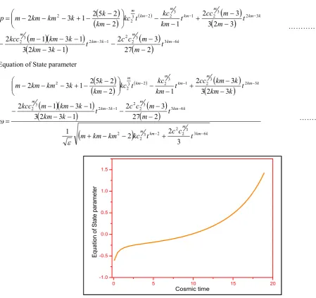
k km m k km m k km m km m km m t m m c c t k km k km m kcc t m m cc t km kc t kc km k k km km m p 6 3 3 2 2 1 3 2 3 2 3 2 3 2 1 3 2 2 3 2 2 2 27 3 2 1 3 2 3 1 3 1 2 3 2 3 3 2 1 2 2 5 2 1 3 2                                   ……….(5.4)

Equation of State parameter









 































km k

m km m k km m k km m k km m km m km m t c c t kc km km m t m m c c t k km k km m kcc t k km k km cc t km kc t kc km k k km km m 6 3 3 2 2 2 3 2 2 6 3 3 2 2 1 3 2 3 2 3 2 3 2 1 3 2 2 3 2 2 3 2 2 1 2 27 3 2 1 3 2 3 1 3 1 2 3 2 3 3 2 1 2 2 5 2 1 3 2                                        





………(5.5)

Figure 4. Equation of state parameter versus cosmic time with the appropriate choice of constants

Equation (5.5) represents the equation of state parameter of the model which is a function of cosmic time. The graphical behavior of the equation of state parameter versus cosmic time is shown in Figure (iv). At the initial stage when the universe starts to expand or accelerate for a small interval of time it has value





0

while for the whole interval of time it is





0

hence the

0 1 2 3 4 5 6

0 10 20 30 40 En er g y de n s ity Cosmic time

0 5 10 15 20

[image:6.595.38.488.317.740.2]

expansion the universe expands with quintessence







1

region, for the whole interval it behaves as like matter-dominated once.

Stability factor of the model

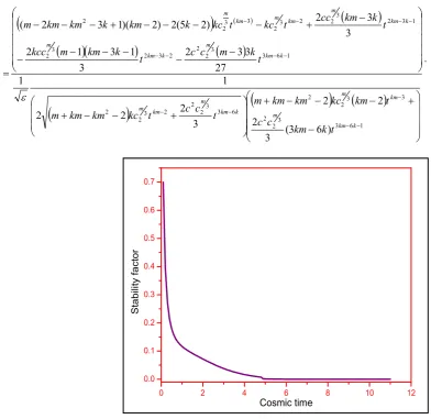
For the stability of corresponding solution, we should check that ourmodels are physically acceptable. For this, firstly it isrequired that the velocity of sound should be less thanvelocity of light i.e. within the range

0





2.

In our derived model, we obtained the sound speed as





 



























                                                                            1 6 3 3 2 2 3 3 2 2 6 3 3 2 2 2 3 2 2 1 6 3 3 2 2 2 3 2 3 2 1 3 2 3 2 2 3 2 3 3 2 2 2 ) 6 3 ( 3 2 2 2 3 2 2 2 1 1 27 3 3 2 3 1 3 1 2 3 3 2 ) 2 5 ( 2 ) 2 )( 1 3 2 ( k km m km m k km m km m k km m k km m k km m km m km m t k km c c t km kc km km m t c c t kc km km m t k m c c t k km m kcc t k km cc t kc t kc k km k km km m  

[image:7.595.46.439.164.545.2]

. ………(5.6)

Figure 5. Stability factor of the model versus cosmic time with the appropriate choice of constants

6. Kinematical Properties of the model

The kinematical properties which are important in cosmology for discussing the geometrical behavior of the universe that are spatial volume, Hubble parameter, expansion scalar, shear scalar and an anisotropic parameter which have the following expressions

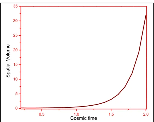
The spatial volume,

t

t

c

V



₂ 3 . ………(6.1)

It is observed that the spatial volume

V

has constant value at an initial time

t



0

, expands exponentially as

t

increases and becomes infinitely large at

t





. Figure (vi) shows the behavior of spatial volume versus cosmic time.

The spatial volume of the Universe starts with a constant value at t → 0, it always expands with an increase in time which shows that the Universe starts evolving with zero volume and expands with time. Thus, inflation is possible in this model.

0 2 4 6 8 10 12

[image:8.595.166.430.50.259.2]

Figure 6. Spatial volume versus cosmic time with an appropriate choice of constants

The mean Hubble parameter,

t

k

H



. …….……….(6.2)

The scalar expansion

t

k

3



[image:8.595.155.437.366.603.2]



. ………..(6.3)

Figure 7. Hubble’s parameter and Expansion scalar versus cosmic time with appropriate choice of constants

At the initial epoch, the Hubble’s parameter and the expansion scalar both are infinitely high and decreases with expansion and at infinite expansion, both are null or approaches zero monotonically. Behavior is clearly shown in figure (vii).

The mean anisotropy parameter,

2 6 2 2 2

9

2

 





t

km k

k

c

. ………...(6.4)

The shear scalar,

4 6 2 2 2

3

 



km k

t

c



. ………...(6.5)

0.5 1.0 1.5 2.0

0 5 10 15 20 25 30 35

Spatia

l Vo

lu

me

Cosmic time

0.0 0.5 1.0 1.5 2.0

0 5 10 15 20 25

30 Hubble's parameter

Expansion scalar

From equations (6.4) and (6.5) the mean anisotropic parameter and shear scalar both are function of time. Initially at

t



0

both are diverges at

t



0

while they becomes vanishes as

t





. Hence, the universe does approach isotropy at infinite expansion.

6. Conclusion

In the investigation of a locally rotationally symmetric spatially homogeneous and anisotropic Bianchi type-I space-time, in the presence of perfect fluid with Quadratic form of Equation of State towards the field equations

f

(

R

)

gravity using volumetric power and exponential law of expansion it is observed that the function of Ricci scalar of the model is positive and decreasing function of time while the Ricci scalar is also positive but initially increases the then decreases with cosmic time. For the whole spreading out initially, the energy density of the model is very high and gradually decreases with the expansion and attend a small positive value. The equation of state parameter of the model which is a function of cosmic

time. At the initial stage when the universe starts to expand or accelerate for a small interval of time, it has value





0

while for the whole interval of time it is





0

hence the expansion the universe expands with quintessence







1

region, for the whole interval it behaves as like matter-dominated once. The spatial volume of the Universe starts with a constant value at t → 0, it always expands with an increase in time which shows that the Universe starts evolving with zero volume and expands with time. Thus, inflation is possible in this model. At the initial epoch, the Hubble’s parameter and the expansion scalar both are infinitely high and decreases with expansion and at infinite expansion, both are null or approaches zero monotonically. The mean anisotropic parameter and shear scalar both are a function of time. Initially, at

t



0

both are diverges at

t



0

while they become vanishes as

t





. Hence, at infinite expansion the universe approach isotropy. From the figure (v) it is observed that the stability factor of the model is initially positive which satisfy that the velocity of sound should be less than the velocity of light i.e. within the range

0





2, but with the expansion it is null. Hence, with the expansion of the model, The Universe is unstable.

7. REFERENCES

Armendariz-Picon C., Mukhanov V., Steinhardt P.:Phys. Rev. D 63 (2001) 103510 Azadi A., Momeni D., Nouri-Zonoz M.: Phys. Lett. B670 (2008) 210-214

Bhoyar S.R., Chirde V.R., Shekh S.H.:3 Inter. J. of Adv. Resea. 3 (9) 492 (2015) Caldwell R., Kamionkowski M., Weinberg N.: Phys. Rev. Lett. 91(2003) 071301 Capozziello S., Martin-Moruno P., Rubano C.: Phys. Lett. B664(2008) 12-15 Chirde V. R., Shekh S. H.: Bulg. J. Phys. 43 156 (2016)

Chirde V.R., Shekh S. H.,:Astrofiz. 58 (2015) 1, 121-133

Chirde V.R., Shekh S. H.: General Relativity and Gravitation (2019) 51:87; https://doi.org/10.1007/s10714-019-2565-7 Chirde V.R., Shekh S. H.: J. Astrophys. Astr. (2016) 37:15DOI: 10.1007/s12036-016-9391-z

Chirde V.R., Shekh S. H.: J. Astrophys. Astr. (2018) 39:56 https://doi.org/10.1007/s12036-018-9555-0 ChirdeV.R., ShekhS.H.:Bulg. J. Phys. 41 258 (2014)

ChirdeV.R., ShekhS.H.:Indian Journal of Physics, 92(11), 1485-1494, 2018 https://doi.org/10.1007/s12648-018-1236-y Einstein A.:(1930) Math. Ann. 102 685.

Harko T.et al.: Phys. Rev. D 84, 024020(2011)

Hinshaw G.et al.:Astrophys. J. Suppl., 180 (2009) 225-245. KatoreS.D., ShaikhA.Y.:Afr.Rev.Phys. 9 (2014) 0055

Miranda V., Joras S, Waga I., Quartin M.:Phys. Rev. Lett. 102 (2009) 221101 Nojiri S.,OdintsovS. :arXiv: 0807.0685 (2008) 266-285

Perlmutter S.et al.:Astrophys. J., 483(1997) 565-581; Perlmutter S.et al.: Nature, 391(1998) 51-54; Perlmutter S.et al.:Astrophys. J., 517 (1999)565-586

Riess A. et al.: Astron. J., 116 (1998)1009-1038.

Rodrigues M.E. et al. arXiv: 1308.(2013) 2962v2 [gr-qc].

Sahoo P., Mishra B., Chakradhar G., Reddy D.: Eur. Phys. J. Plus 129, 49 (2014) SetareM.R. et al. arXiv: 1203.(2013) 1315v3 [gr-qc].

Sharif M., Shamir M.: Gen. RelaOv. Gravit. 42 1557 (2010) Sharif M., Yousaf Z. J. Cosmo. :Astropart. Phys. (2014)06- 019 Sharif M., Azeem S.: Astrophys. Space Sci. 342 (2012521-530. Spergel D.et al.: Astrophys. J. Suppl.,148 (2003)175-194. Steinhardt P., Wang L., Zlatev I. :Phys. Rev. D 59(1999) 123504 Turner M.: Astro-ph(2001) /0108103

Uddin K., Lidsey J., Tavakol R.: Class. Quant. Gravit. 24, 3951 (2007) Verde L.et. al., Mon. Not. R.: Astron. Soc., 335 (2002) 432-440;

Zlatev I., Wang L., Steinhardt P.:Phys. Rev. Lett. 82 (1999) 896-899