16
Explaining non-linear Classifier Decisions
within Kernel-based Deep Architectures
Danilo Croce and Daniele Rossini and Roberto Basili Department of Enterprise Engineering
University of Roma, Tor Vergata
{croce,basili}@info.uniroma2.it
Abstract
Nonlinear methods such as deep neural net-works achieve state-of-the-art performances in several semantic NLP tasks. However episte-mologically transparent decisions are not pro-vided as for the limited interpretability of the underlying acquired neural models. In neural-based semantic inference tasks epistemologi-cal transparency corresponds to the ability of tracing back causal connections between the linguistic properties of a input instance and the produced classification output.
In this paper, we propose the use of a method-ology, called Layerwise Relevance Propaga-tion, over linguistically motivated neural ar-chitectures, namelyKernel-based Deep Archi-tectures(KDA), to guide argumentations and explanation inferences. In such a way, each decision provided by a KDA can be linked to real examples, linguistically related to the in-put instance: these can be used to motivate the network output. Quantitative analysis shows that richer explanations about the semantic and syntagmatic structures of the examples charac-terize more convincing arguments in two tasks, i.e. question classification and semantic role labeling.
1 Introduction
Nonlinear methods such as deep neural networks achieve state-of-the-art performances in several challenging problems, such as image classification or natural language processing (NLP). However the traditional AI criticism still holds: they are not epistemologically transparent, as for the limited interpretability of the neural inferences.
In a question classification (QC) task, e.g. (Li and Roth, 2006), this is particularly evident. The category describing the target of a request is rel-evant in question answering to optimize the later
stages of search and answer detection, and its in-terpretation depends on a variety of semantic and syntactic properties of the question. Epistemolog-ical transparency corresponds here to the ability of tracing back the connections between linguistic properties of the input question and the proposed question category. An example-driven machine learning model should be able to provide causal re-lations between the input semantic aspect and the properties of the question.
For example, given the prediction ”What is the capital of Zimbabwe?”refers to aLocation, we would like the system to motivate it with a sen-tence such as: Since it seems similar to ”What is the capital of California?” which also refers to a
Location.
Notice how in neural learning, as for exam-ple in Multilayer Perceptrons, Long Short-Term Memory Networks, (Hochreiter and Schmidhuber, 1997), or the more recent Attention-based Net-works (Larochelle and Hinton,2010), the network parameters have no clear conceptual counterpart.
Using the Layerwise Relevance Propagation
(LRP) (Bach et al., 2015) approach, the classi-fication decisions of a multilayer perceptron are decomposed backward across the network layers, and evidence about the contribution of individual input fragments (i.e. layer 0) to the final decision is gathered. Evaluation against images (i.e. the MNIST and ILSVRC data sets) suggests that LRP activates meaningful associations between input and output fragments, and this corresponds to trac-ing back meantrac-ingful causal connections.
2001) within neural-based learning. Here, we show that the inferences of such architectures can be motivated by simply applying the LRP method, which allows to trace back causal as-sociations between the semantic classification and the examples expressed by parse tree-based metrics. Evaluation of the LRP algorithm to the problem of explaining the system decisions allows to demonstrate the meaningful impact of LRP on semantic transparency: users faced with explanations are better oriented to accept or reject the system decisions, thus improving the impact on the overall application accuracy.
In the rest of the paper, section 2 reports re-lated works. In section3we describe the Kernel-based Deep Architecture (KDA) while section 4 illustrates the details of LRP and how it connects to KDAs. In section 5 we propose both a novel model to generate explanations of a network pre-diction and an evaluation methodology. In section 6we provide experimental evidences of the overall system’s effectiveness against two semantic tasks, question classification and frame-based argument classification in the semantic role labeling chain. Lastly, in section7conclusions are derived.
2 Related Work
Linguistically motivated explanatory methods
should provide semantically clear justifications about a neural network textual inferences.
Methods making the neural learning more read-able are usually designed to trace back the por-tions of the network input that mostly contributed to the output decision. Network propagation tech-niques are used to identify the patterns of a given input item (e.g., an image) that are linked to the particular deep neural network prediction as in (Erhan et al.,2010;Zeiler and Fergus,2013). Usu-ally, these are based on backward algorithms that layer-wise reuse arc weights to propagate the pre-diction from the output down to the input, thus leading to the re-creation ofmeaningfulpatterns in the input space. Typical examples are deconvolu-tion heatmaps, used to approximate through Tay-lor series the partial derivatives at each layer (Si-monyan et al.,2013), or the so-called Layer-wise Relevance Propagation (LRP), that redistributes back positive and negative evidence across the lay-ers (Bach et al.,2015).
Several efforts have been made in the
perspec-tive of providing explanations of a neural classi-fier, often by focusing into highlighting an handful of crucial features (Baehrens et al.,2010) or deriv-ing simpler, more readable models from a complex one, e.g. a binary decision tree (Frosst and Hinton, 2017), or by local approximation with linear mod-els (Ribeiro et al.,2016). However, although they can explicitly show the representations learned in the specific hidden neurons (Frosst and Hinton, 2017), these approaches base their effectiveness on the user ability to study the quality of the rea-soning and of the accountability as a side effect of the quality of the selected features: this can be very hard in tasks where boundaries between classes are not well defined. Sometimes, explana-tions are associated to vector representaexplana-tions as in (Ribeiro et al.,2016), i.e. bag-of-word in case of text classification, which is clearly weak at captur-ing significant lcaptur-inguistic abstractions, such as the involved syntactic relations. In this work, we pro-pose a model which allows to provide explanations that are easily interpretable even by non-expert users, as they are expressed in natural language and are hence a more natural solution. It implicitly captures lexical, semantic and syntactic general-izations through the generation of a linguistically fluent explanation of predictions: as this is exploit linguistic analogies it provides a more transparent and epistemologically coherent view on the sys-tem’s decision.
3 A Kernel-based Deep Architecture
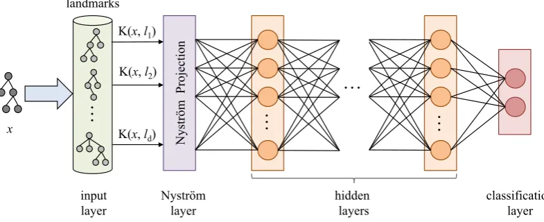
In this section, we will first describe the Nystr¨om method for generating low dimensional embed-dings that approximate high dimensional kernel spaces. Then we will review the Kernel-based Deep Architecture discussed in (Croce et al., 2017), that efficiently combines kernel methods and deep learning by using a Nystr¨om layer into a neural architecture.
N
ys
tröm
P
roj
ec
ti
on
…
…
…
K(x, l1)
K(x, l2)
K(x, ld)
hidden layers
classification layer landmarks
…
Nyström layer input
layer
[image:3.595.97.490.69.229.2]x
Figure 1: Kernel-based Deep Architecture.
X. The Gram matrix can always be computed as G=XX>, with each single element corre-sponding toGij = Φ(oi)Φ(oj) = K(oi, oj). The aim of the Nystr¨om method is to derive a new low-dimensional embeddingx˜ in al-dimensional space, withlnso thatG˜ = ˜XX˜>andG˜ ≈G. This is obtained by generating an approximation
˜
GofGusing a subset oflcolumns of the matrix, i.e., a selection of a subset L ⊂ D of the avail-able examples, calledlandmarks. Suppose we ran-domly samplelcolumns ofG, and letC ∈R|D|×l be the matrix of these sampled columns. Then, we can rearrange the columns and rows ofGand de-fineX= [X1 X2]such that:
G=XX>=
W X1>X2 X2>X1 X2>X2
and C=
W X2>X1
whereW =X1>X1, i.e., the subset ofGthat con-tains only landmarks. The Nystr¨om approxima-tion can be defined as:
G≈G˜ =CW†C> (1)
whereW† denotes the Moore-Penrose inverse of W. The Singular Value Decomposition (SVD) is used to obtainW† as it follows. First, W is de-composed so that W = U SV>, where U and V are both orthogonal matrices, and S is a di-agonal matrix containing the (non-zero) singular values of W on its diagonal. Since W is sym-metric and positive definite, W = U SU>. Then W†=U S−1U>=U S−12S−
1
2U>and the
Equa-tion1can be rewritten as
G≈G˜=CU S−12S− 1 2U>C>
= (CU S−12)(CU S− 1
2)>= ˜XX˜>
Given an input example o ∈ D, a new low-dimensional representation ~x˜ can be thus deter-mined by considering the corresponding item of Cas
˜
~x=~cU S−12 (2)
where~c is the vector whose dimensions contain the evaluations of the kernel function between o and each landmarkoj ∈L. Therefore, the method producesl-dimensional vectors.
Notice that an optimal selection of landmarks can be expected to reduce the Gram Matrix ap-proximation error. However, the uniform sam-pling without replacement policy is adopted: it is in fact theoretically and empirically shown in Kumar et al. (2012) to achieve results compara-ble with alternative but (more complex) selection policies.
In (Croce et al., 2017), the Nystr¨om represen-tation~x˜has been used as input within neural net-work architectures. In fact, given a labeled dataset L = {(o, y) |o ∈ D, y ∈ Y}, whereo refers to a generic instance andyis its associated class, a Multi-Layer Perceptron (MLP) architecture can be defined, with a specific Nystr¨om layer based on the Nystr¨om embeddings of Eq. 2. Such Kernel-based Deep Architecture (KDA) has an in-put layer, a Nystr¨om layer, a possibly empty se-quence of non-linear hidden layers and a final
The input layer corresponds to the input vec-tor~c, i.e., the row of the C matrix associated to an exampleo. The input layer is mapped to the
Nystr¨om layer, through the projection in Equa-tion 2. Notice that the embedding provides also the proper weights, defined byU S−12, so that the
mapping can be expressed through the Nystr¨om matrix HN y=U S−
1
2: it corresponds to a
pre-trained stage derived through SVD. Formally, the low-dimensional embedding of an input example o, is~x˜=~c HN y=~c U S−
1 2.
The resulting outcome~x˜ is the input to one or more non-linear hiddenlayers. Each t-th hidden layer is realized through a matrixHt∈Rht−1×ht and a bias vector~bt ∈ R1×ht, where ht denotes the desired hidden layer dimensionality. Clearly, given that HN y ∈ Rl×l, h0 = l. The first hid-den layer in fact receives in input ~x˜ = ~cHN y, that corresponds to thet = 0layer input~x0 = ˜~x and its computation is formally expressed by ~
x1 =f(~x0H1+~b1), where f is a non-linear ac-tivation function. In general, the generict-th layer is modeled as:
~
xt=f(~xt−1Ht+~bt) (3)
The final layer of KDA is the classification layer, realized through the output matrixHO and the output bias vector~bO. Their dimensionality depends on the dimensionality of the last hidden layer (calledO−1) and the number|Y|of different classes, i.e., HO ∈ RhO−1×|Y|and~b
O∈R1×|Y|, respectively. In particular, this layer computes a linear classification function with a softmax oper-ator so thatyˆ=sof tmax(~xO−1HO+~bO).
In addition to standard dropout, aL2 regulariza-tion is applied to the norm of each layer.
Finally, the KDA is trained by optimizing a loss function made of the sum of two factors: first, the cross-entropy function between the gold classes and the predicted ones; second theL2 regulariza-tion, whose importance is regulated by a meta-parameterλ. The final loss function is thus
L(y,yˆ) = X (o,y)∈L
y log(ˆy)+λ X H∈{Ht}∪{HO}
||H||2
whereyˆare the softmax values computed by the network andy are the true one-hot encoding val-ues associated with the example from the labeled training datasetL.
As shown in Figure 1, it is worth noticing that the network is stimulated with an input vector c
which contains the kernel evaluationsK(s, li) be-tween each example and the landmarks. When using linguistic kernels (such as Semantic Tree Kernels) this measure corresponds to a syntac-tic/semantic similarity between thexand the sub-set of examples used for the space reconstruction (made available through the Nystr¨om method). Once stimulated, the network will provide an out-put. In order to give an explanation to a network decision, we will discuss in the following section how to revert the propagation process connecting output and input. As a side effect we will be able to determine those landmarks mostly affecting the final decision and which are more semantically re-lated to the input instance.
4 Layer-wise Relevance Propagation in Kernel-based Deep Architectures
Layer-wise Relevance propagation (LRP, pre-sented in (Bach et al.,2015)) is a framework which allows to decompose the prediction of a deep neu-ral network computed over a sample, e.g. an im-age, down to relevance scores for the single input dimensions of the sample such as subpixels of an image.
More formally, let f : Rd → R+ be a posi-tive real-valued function taking a vector x ∈ Rd as input. The functionf can quantify, for exam-ple, the probability of x being in a certain class. The Layer-wise Relevance Propagation assigns to each dimension, or feature, xd a relevance score R(1)d such that:
f(x)≈P dR
(1)
d (4)
Features whose score is R(1)d > 0 or R(1)d < 0 correspond to evidence in favor or against, respec-tively, the output classification. In other words, LRP allows to identify fragments of the input play-ing key roles in the decision, by propagatplay-ing rele-vance backwards. Let us suppose to know the rel-evance scoreR(jl+1)of a neuronjat network layer l+ 1, then it can be decomposed into messages R(il,l←+1)j sent to neuronsiin layerl:
Rj(l+1) = X i∈(l)
R(i←l,l+1)j (5)
Hence it derives that the relevance of a neuroniat layerlcan be defined as:
R(il)= X j∈(l+1)
Note that 5 and6 are such that4 holds. In this work, we adopted the-rule defined in (Bach et al., 2015) to compute the messagesR(i←l,l+1)j :
Ri(←l,l+1)j = zij zj+·sign(zj)
Rj(l+1)
wherezij = xiwij and > 0is a numerical sta-bilizing term and must be small. The informative value is justified by the fact that the weights zij are linked to the activation weightswij of the in-put neurons.
If we apply it to a KDA processing linguistic ob-servations, then LRP implicitly traces back the syntactic, semantic and lexical relations between the example and the landmarks, thus it selects the landmarks whose presences were the most influ-ential to identify the predicted structure in the sen-tence. Indeed, each landmark is uniquely associ-ated to an entry of the input vector~c, as illustrated in Sec3.
5 Explanatory Models
Justifications for the KDA emissions can be ob-tained by explaining the evidence in favour or against a class using landmarks{`}as examples. The idea is to select those{`}that the LRP method produces as the most active elements in layer 0. Once such active landmarks are detected, an Ex-planatory Model is a function in charge to com-pile the linguistically fluent explanation by using analogies or differences with the input case. The semantic expressiveness of such analogies makes the resulting explanation clear and increases the user confidence on the system reliability. When a sentence sis classified, LRP assigns activation scoresr`sto each individual landmark`: letL(+) (orL(−)) denote the set of landmarks with positive (or negative) activation score.
Formally, every explanation is characterized by a triplee=hs, C, τiwheresis the input sentence, Cis the predicted label andτis the modality of the explanation:τ = +1for positive (i.e. acceptance) statements whileτ =−1correspond to rejections of the decisionC.
A landmark ` is positively activated for a given sentencesif there are not more thank−1other ac-tive landmarks`0whose activation value is higher than the one for`, i.e.
|{`0 ∈ L(+):`06=`∧rs
`0 ≥r`s>0}|< k
Similarly, a landmark is negatively activated
when:
|{`0 ∈ L(−) :`06=`∧rs
`0 ≤r`s<0}|< k
where k is a parameter used to make explana-tion depending on not more thanklandmarks, de-noted byLk. Positively (or negative) active land-marks in Lk are assigned to an activation value a(`, s) = +1 (−1), whilea(`, s) = 0for all other not activated landmarks.
Given the explanatione=hs, C, τi, a landmark `whose (known) class is C` isconsistent (or
in-consistent) with e according to the fact that the following function:
δ(C`, C)·a(`, q)·τ
is positive (or negative, respectively), where δ(C0, C) = 2δkron(C0 =C)−1andδkronis the Kronecker delta.
An explanatory model is then a function M(e,Lk)which maps an explanatione, a sub set Lkof the activeandconsistent landmarksLfore into a sentencef in natural language. Of course several definitions forM(e,Lk) are possible. A general explanatory model would be:
M(e,Lk) =
’sisCsince it is similar to`’ ∀`∈ L+k ifτ >0
’sis notCsince it is different from`which isC’
∀`∈ L−k ifτ <0
’sisCbut I don’t know why’ ifL ≡ ∅
whereL±k are the partition of landmarks with pos-itive and negative relevance scores inLk, respec-tively.
Here we introduce three explanatory models we used during experimental evaluation:
I think”this plate”isTHEMEof PLACINGin ”Robot
PUTthis platein the center of the table” since similar to
”the soap”in ”Can youPUTthe soapin the washing
machine?”.
(Multiplicative Model) In a second model, de-noted as multiplicative, the system makes refer-ence to up to k1 ≤ k analogies with positively (or negatively) active and consistent landmarks. Given the above explanation e1, and k1 = 2, it would return:
I think”this plate”isTHEMEof PLACINGin ”Robot
PUTthis platein the center of the table” since similar to
”the soap”in ”Can youPUT”the soap”in the washing
machine?” and it is also similar to”my coat”in ”HANGmy
coatin the closet in the bedroom”.
(Contrastive Model) The last proposed model is more complex since it returns both a positive (whetherτ = 1) and a negative (τ =−1) analogy by selecting, respectively, the most positively rel-evant and the most negatively relrel-evant consistent landmark: For instance, givene1, it could return:
I think”this plate”is theTHEMEof PLACINGin ”Robot
PUTthis platein the center of the table” since similar to
”the soap”which is in ”Can youPUTthe soapin the
washing machine” and it is not theGOALof PLACING
since different from”on the counter” in ”PUTthe plateon
the counter”.
5.1 Using information theory for validating explanations
Let P(C|s) and P(C|s, e) be, respectively, the prior probability of the classification of s being correct and the probability of the classification be-ing correct given an explanation. Note that both indicate the level of confidence the user has in the classifier (i.e. the KDA) given the amount of avail-able information, i.e. with and without explana-tion. Three explanations are possible:
• Useful explanations: these are explanations such that C is correct and P(C|s, e) > P(C|s)orC is not correct andP(C|s, e) < P(C|s)
• Useless explanations: they are explanations such thatP(C|s, e) =P(C|s)
• Misleading explanations:they are explana-tions such thatCis correct andP(C|s, e) < P(C|s)orC is not correct andP(C|s, e) > P(C|s)
The core idea is that semantically coherent and ex-haustive explanations must indicate correct clas-sifications whereas incoherent or non-existent ex-planations must hint towards wrong classifica-tions.
Given the above probabilities, we can mea-sure the quality of an explanation by computing the achieved Information Gain (Kononenko and Bratko, 1991): the posterior probability is ex-pected to grow w.r.t. to the prior one for cor-rect decisions when a good explanation is avail-able against the input sentence, while decreas-ing for bad or confusdecreas-ing explanations. The intu-ition behind Information Gain is that it measures the amount of information (provided in number of bits) gained by the explanation about the user decision of accepting the system classification on an incoming sentences. A positive gain indicates that the probability amplifies towards the right de-cisions, and declines with errors. We will let users to judge the quality of the explanation and assign them a posterior probability that increases along with better judgments. In this way we have a mea-sure of how convincing the system is about its de-cisions as well as how weak it is to clarify erro-neous cases. To compare the overall performance of the different explanatory modelsM, the Infor-mation Gain is measured against a collection of explanations generated byM and then normalized throughout the collection’s entropyEas follows:
Ir= 1 E
1 | Ts|
|Ts|
X
j=1
I(j) = Ia
E (7)
whereTsis the explanations collection andI(j)is the Information Gain of explanationj.
6 Experimental Evaluation
The effectiveness of the proposed approach has been measured against two different semantic pro-cessing tasks,i.e. question classification and argu-ment classification in semantic role labeling. The Nystrom projection has been implemented in the KeLP framework (Filice et al.,2018)1, the neural network and LRP have been implemented in Ten-sorflow2, with 1 and 2 hidden layers, respectively, whose dimensionality corresponds to the number of involved Nystrom landmarks (500 and 200,
re-1
http://www.kelp-ml.org
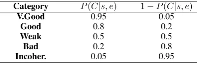
Category P(C|s, e) 1−P(C|s, e)
V.Good 0.95 0.05
Good 0.8 0.2
Weak 0.5 0.5
Bad 0.2 0.8
Incoher. 0.05 0.95
Table 1: Posterior probabilities w.r.t. quality categories
Class Incoher. Bad Weak Good V.Good
Incoher. 1.00 0.83 0.50 0.16 0.00
Bad 0.83 1.00 0.66 0.33 0.16
Weak 0.50 0.66 1.00 0.66 0.50
Good 0.16 0.33 0.66 1.00 0.83
[image:7.595.82.280.61.124.2]V.Good 0.00 0.16 0.50 0.83 1.00
Table 2: Weights for the Cohen’s Kappaκwstatistics
spectively, randomly selected3), and the adoption of dropout regularization in hidden and final lay-ers. For both tasks, hyper-parameters have been optimized via grid-search. The Adam optimizer has been applied to minimize the cross-entropy loss function, with a multi-epoch (500) training, each fed with batches of size 256. We adopted an early stop strategy, where the best model was selected according to the performance over the de-velopment set.
For evaluating our explanation method, we de-fined five quality categories and associated them to values for the posteriori probabilityP(C|s, e), as shown in Table 1. We gathered into explana-tion datasets hundreds of explanaexplana-tions from the three models for each task and presented them to a pool of annotators (further details in related sub-sections) for independent labeling; annotators had no information of the correctness of the system emissions but just knowledge about the dataset en-tropy. We addressed their consensus by measuring a weighted Cohen’s Kappa.
6.1 Question Classification
In our first evaluation, we replicated the experi-ments reported by (Croce et al.,2017) with respect to the question classification task. We thus used the UIUC dataset (Li and Roth, 2006), including a training and test set of5452and500questions, respectively, organized in 6 coarse-grained classes
(as ENTITY orHUMAN). We generated Nystrom
representation of the Compositionally Smoothed Partial Tree Kernel (Annesi et al.,2014) function with default parametersµ =λ= 0.4. Using 500
3More complex policies have been applied to select
land-marks but statistically significant results have not been mea-sured (not reported here due to space limitations).
QC SRL-AC
Basic 0.548 0.669
Multiplicative 0.514 0.662
Contrastive 0.576 0.667
κw 0.677 0.783
accuracy 0.926 0.961
Table 3: Information gains for the three Explanatory Models applied to the SRL-AC and QC datasets.kwis
the weighted Cohen’s Kappaκw.
landmarks, the KDA accuracy was92.6%. A group of 3 annotators evaluated an explanation dataset of 300 explanations (perfectly balanced be-tween correct and not correct classification), com-posed of 100 explanations for each model. Perfor-mances are shown in Table3.
All three explanatory models were able to gain more than half the required information in order to ascertain the correctness of the classification. Consider:
I think ”What year did Oklahoma become a state ?” refers to aNUMBERsince similar to ”The film Jaws was made in
what year ?”
The model provided an evidently coherent anal-ogy, but this is a easy case due to the occurrence in both questions of very discriminative words, i.e
”what year”. However, the system is also able to capture semantic similarities when both syntactic and lexical features are different. E.g.:
I think ”Where is the Mall of the America ?” refers to a
LOCATIONsince similar to ”What town was the setting for
The Music Man ?”.
This is an high-quality explanation since the sys-tem provided an analogy with a landmark request-ing the same fine-grained category but with little sharing of lexical and syntactic information (note, for example, the absence in the landmark of the very discriminative word ”where”). Let us now consider the case of wrong classifications:
I think ”Mexican pesos are worth what in U.S. dollars ?”
refers to aDESCRIPTION since similar to ”What is the
Bernoulli Principle ?”
The system provided an explanation that is not possible to easily interpret: indeed it was labeled as [Incoherent] by all the annotators.
[image:7.595.313.518.61.125.2]I think ”What is angiotensin ?” does not refer to aNUM
since different from ”What was Einstein ’s IQ ?”.
is correct but obvious. As an alternative, a nega-tive analogy with a very likely class, i.e.ENTITY
or DESCRIPTION, would have provided more
useful information for disambiguation. A second challenge is represented by inherently ambiguous questions. The following explanation
I think ”What is the sales tax in Minnesota ?” refers to a
NUMBERsince similar to ”What is the population of
Mozambique ?” and does not refer to a ENTITYsince
different from ”What is a fear of slime ?”.
tells why NUMBER is a more likely class than
ENTITY. Although seemingly correct, this is a
mistake, asENTITYis the proper decision. How-ever, the explanation is perfectly fine, as it well expresses the decision’s rationale: lack of contex-tual information in the question is here the main cause of the error.
6.2 Argument Classification
Semantic role labeling (SRL (Palmer et al.,2010)) consists in detecting the semantic arguments asso-ciated with the predicate of a sentence and their classification into their specific roles (Fillmore (1985)). For example, given the sentence ”Bring the fruit onto the dining table”, the task would be to recognize the verb ”bring” as evoking the BRINGING frame, with its roles, THEMEfor ”the fruit” and GOAL for ”onto the dining table”. Ar-gument classification corresponds to the subtask of assigning labels to the sentence fragments span-ning individual roles.
As proposed in (Moschitti et al., 2008), SRL can be modeled as a multi classification task over each parse tree noden, where argument spans re-flect sub-sentences covered by the tree rooted at
n. Consistently with (Croce et al., 2011), in our experiments the KDA has been empowered with a Smoothed Partial Tree Kernel, operating over Grammatical Relation Centered Tree (GRCT) de-rived from dependency grammar.
We used the HuRIC dataset (Bastianelli et al., 2014), including over 650 annotated transcrip-tions of spoken robotic commands, organized in 18frames and about60arguments4. We extracted single arguments from each HuRIC example, for a total of1,300instances. We run experiments with a methodology similar to the one described in Sec
4http://sag.art.uniroma2.it/lu4r.html
6.1, but due to the limited data size we performed extensive 10-fold cross-validation, optimizing net-work hyper-parameters via grid-search for each test set. We generated Nystrom representation of a equally-weighted linear combination of SPTK function with default parametersµ=λ= 0.4and of linear kernel function applied to sparse vector representing the instance frame. With these set-tings, the KDA accuracy was 96.1%. We sam-pled 692 explanations almost equally distributed among the 3 explanatory models. Two annotators were involved.
Results are shown in Tab 3. In this task, all models were able to gain more than two thirds of needed information. The alike scores of the three models are probably due to the narrow linguistic domain of the corpus and the well-defined seman-tic boundaries between the arguments. To show the capability of such models, let us consider:
I think”the washer”is the CONTAINING OBJECTof
CLOSUREin ”Robot can youOPENthe washer?” since
similar to”the jar”in ”CLOSEthe jar” and it is not the
THEME of BRINGINGsince different from”the jar”in ”TAKEthe jarto the table of the kitchen”.
I think”me”is the BENEFICIARYof BRINGINGin ”I
would like some cutlery can youGETmesome?” since
similar to”me”in ”BRINGmea fork from the press.” and it
is not the COTHEMEof COTHEMEsince different from
”me”in ”Would you pleaseFOLLOWmeto the kitchen?”.
The above commands have very limited lexical overlap with retrieved landmarks. Nevertheless, the analogies make explanations quite effective: explanatory models seems to successfully capture semantic and syntactic relations among input in-stances and closely related landmarks.
7 Conclusion
References
Paolo Annesi, Danilo Croce, and Roberto Basili. 2014. Semantic compositionality in tree kernels. In Pro-ceedings of CIKM 2014. ACM.
Sebastian Bach, Alexander Binder, Gregoire Mon-tavon, Frederick Klauschen, Klaus-Robert Mller, and Wojciech Samek. 2015. On pixel-wise explana-tions for non-linear classifier decisions by layer-wise relevance propagation. PLOS ONE, 10(7).
David Baehrens, Timon Schroeter, Stefan Harmel-ing, Motoaki Kawanabe, Katja Hansen, and Klaus-Robert M¨uller. 2010. How to explain individ-ual classification decisions. J. Mach. Learn. Res., 11:1803–1831.
Emanuele Bastianelli, Giuseppe Castellucci, Danilo Croce, Luca Iocchi, Roberto Basili, and Daniele Nardi. 2014. Huric: a human robot interaction cor-pus. In LREC, pages 4519–4526. European Lan-guage Resources Association (ELRA).
Michael Collins and Nigel Duffy. 2001. New rank-ing algorithms for parsrank-ing and taggrank-ing: Kernels over discrete structures, and the voted perceptron. In Pro-ceedings of the 40th Annual Meeting on Association for Computational Linguistics (ACL ’02), July 7-12, 2002, Philadelphia, PA, USA, pages 263–270. Asso-ciation for Computational Linguistics, Morristown, NJ, USA.
Danilo Croce, Simone Filice, Giuseppe Castellucci, and Roberto Basili. 2017. Deep learning in seman-tic kernel spaces. InProceedings of the 55th Annual Meeting of the Association for Computational Lin-guistics (Volume 1: Long Papers), pages 345–354, Vancouver, Canada. Association for Computational Linguistics.
Danilo Croce, Alessandro Moschitti, and Roberto Basili. 2011. Structured lexical similarity via convo-lution kernels on dependency trees. InProceedings of EMNLP ’11, pages 1034–1046.
Dumitru Erhan, Aaron Courville, and Yoshua Ben-gio. 2010. Understanding representations learned in deep architectures. Technical Report 1355, Univer-sit´e de Montr´eal/DIRO.
Simone Filice, Giuseppe Castellucci, Giovanni Da San Martino, Alessandro Moschitti, Danilo Croce, and Roberto Basili. 2018. Kelp: a kernel-based learning platform. Journal of Machine Learning Research, 18(191):1–5.
Charles J. Fillmore. 1985. Frames and the semantics of understanding. Quaderni di Semantica, 6(2):222– 254.
Nicholas Frosst and Geoffrey Hinton. 2017. Distilling a neural network into a soft decision. CEUR Work-shop Proceedings, 2071.
Sepp Hochreiter and J¨urgen Schmidhuber. 1997. Long short-term memory. Neural Comput., 9(8):1735– 1780.
Igor Kononenko and Ivan Bratko. 1991. Information-based evaluation criterion for classifier’s perfor-mance.Machine Learning, 6(1):67–80.
Sanjiv Kumar, Mehryar Mohri, and Ameet Talwalkar. 2012. Sampling methods for the nystr¨om method. J. Mach. Learn. Res., 13:981–1006.
Hugo Larochelle and Geoffrey E. Hinton. 2010. Learn-ing to combine foveal glimpses with a third-order boltzmann machine. InProceedings of Neural In-formation Processing Systems (NIPS), pages 1243– 1251.
Xin Li and Dan Roth. 2006. Learning question clas-sifiers: the role of semantic information. Natural Language Engineering, 12(3):229–249.
Alessandro Moschitti, Daniele Pighin, and Roberto Basili. 2008. Tree kernels for semantic role label-ing.Computational Linguistics, 34.
M.S. Palmer, D. Gildea, and N. Xue. 2010. Seman-tic Role Labeling. Online access: IEEE (Institute of Electrical and Electronics Engineers) IEEE Mor-gan & Claypool Synthesis eBooks Library. MorMor-gan & Claypool Publishers.
Marco T´ulio Ribeiro, Sameer Singh, and Carlos Guestrin. 2016. ”why should I trust you?”: Ex-plaining the predictions of any classifier. CoRR, abs/1602.04938.
John Shawe-Taylor and Nello Cristianini. 2004. Ker-nel Methods for Pattern Analysis. Cambridge Uni-versity Press, Cambridge, UK.
Karen Simonyan, Andrea Vedaldi, and Andrew Zisser-man. 2013. Deep inside convolutional networks: Vi-sualising image classification models and saliency maps. CoRR, abs/1312.6034.