Software and methods for oligonucleotide and cDNA array data analysis

comment

reviews

reports

deposited research

interactions

information

refereed research

Software report

Software and methods for oligonucleotide and cDNA array

data analysis

Matthew A Zapala, Daniel J Lockhart, Daniel G Pankratz, Anthony J Garcia,

Carrolee Barlow and David J Lockhart

Address: The Salk Institute for Biological Studies, Laboratory of Genetics, 10010 North Torrey Pines Road, La Jolla, CA 92037, USA.

Correspondence: David J Lockhart. E-mail: dlockhart@ambitbio.com

Abstract

Two HTML-based programs were developed to analyze and filter gene-expression data: ‘Bullfrog’ for Affymetrix oligonucleotide arrays and ‘Spot’ for custom cDNA arrays. The programs provide intuitive data-filtering tools through an easy-to-use interface. A background subtraction and normalization program for cDNA arrays was also built that provides an informative summary report with data-quality assessments. These programs are freeware to aid in the analysis of gene-expression results and facilitate the search for genes responsible for interesting biological processes and phenotypes. Published: 23 May 2002

GenomeBiology2002, 3(6):software0001.1–0001.9

The electronic version of this article is the complete one and can be found online at http://genomebiology.com/2002/3/6/software/0001 © 2002 Zapala et al., licensee BioMed Central Ltd

(Print ISSN 1465-6906; Online ISSN 1465-6914)

Rationale

Microarray technology has radically changed the way researchers address many biological questions. It is now possible to measure messenger RNA levels quantitatively for thousands of genes, or even entire genomes, using DNA arrays, microarrays or ‘chips’ [1,2]. Researchers can, in a fairly straightforward fashion, examine the overall transcrip-tional response of thousands of genes in normal cells and tissues, in disease states, in response to biological, genetic or chemical stimuli (such as drugs), or during normal biological processes such as cell-cycle progression and embryonic development [3-5].

Two of the most commonly used microarrays for gene-expression measurements are oligonucleotide GeneChip® expression arrays made by Affymetrix and custom-made cDNA arrays. Affymetrix oligonucleotide arrays are created by a combination of DNA synthesis and photolithographic tech-niques, whereas cDNA arrays are constructed by spotting or printing PCR products or oligonucleotides onto glass slides [6-9]. Affymetrix arrays contain sets of multiple 25mer oligonucleotide probes specific for each gene or expressed-sequence tag (EST), whereas spotted arrays generally contain

longer cDNA probes (usually 500 to 1,000 bases) or oligo-nucleotide probes (usually 25 to 60 bases) for each gene.

The large amount of information generated from microarrays has been a great strength, but is sometimes seen as a frustrat-ing weakness [10]. A significant obstacle in microarray research has been the inability to process experimental data easily, assess the data quality, manage multiple data sets and mine the data with user-friendly tools that can be quickly learned and applied for routine analysis by laboratory scientists [11].

several seconds. They were created to provide the bench researcher with uncomplicated tools that help focus microarray data from thousands of genes to a relatively small number of high-confidence, differentially expressed candidates. The programs are not intended for high-level statistical or other complex analyses, but they do make it easy to export filtered data to GeneSpring¥or other visual-ization and clustering programs. Lastly, the programs are freeware, made publicly available to the research community in the hope of accelerating functional genomics research.

Manipulating data sets in Bullfrog

Bullfrog and Spot can be used to select genes (probes, probe sets or spots) that behave in specific ways across multiple experiments by using a combination of more than 20 differ-ent qualitative and quantitative criteria (Figure 1). To illus-trate a few of Bullfrog’s capabilities, we use data obtained in gene-expression studies of the adult mouse brain using Affymetrix oligonucleotide arrays [12]. A simple question to ask is, “what genes are differentially expressed between two different regions of the brain (for example, the cerebellum and the amygdala) in a 129S6/SvEvTac (129SvEv) inbred mouse strain?” As in most experiments, it is important to

first estimate the false-positive rate for this type of compari-son between brain regions. The best way to realistically approximate the false-positive rate is to perform and analyze independent experimental replicates of the same brain region from multiple different mice. We used RNA from the cerebellums of two different mice with samples prepared separately and hybridized to two different chips. Ideally, replicate comparisons from well-controlled experiments would show no differentially expressed genes. However, experimental noise and biological variation may lead to genes being scored as differentially expressed between repli-cates. For example, small differences in the brain dissections or differences in the exact time of sacrifice can affect gene-expression patterns. It is very important to estimate the false-positive rate for the particular experimental system being studied, and to set analysis filter criteria that lead to appropriate levels of false positives without sacrificing sensi-tivity to low-abundance mRNA transcripts or subtle changes in gene expression.

To estimate the false-positive rate, a comparison between the data for independent replicate 129SvEv cerebellums was made (that is, expression data from mouse 1 cerebellum versus expression data from mouse 2 cerebellum). This

Figure 1

comparison file (saved as text from the Affymetrix GeneChip®_{MAS 4.0 software) was loaded into Bullfrog and} the filter criteria were selected. A number of different crite-ria may be selected, but our default critecrite-ria for calling a gene ‘differentially expressed’ are as follows: a qualitative differ-ence call of ‘Increase’ (I), ‘Marginal Increase’ (MI), ‘Decrease’ (D) or ‘Marginal Decrease’ (MD), a fold change (expression ratio) of greater than 1.8, an average difference change of greater than 50 (after scaling to a mean signal, or target value, across the entire array of 200), and an absolute call of ‘Present’ for the probe set in either or both replicate cerebellums. The use of multiple filter criteria reduces the risk of erroneously assigning a gene as differentially expressed, while maintaining sensitivity to rare mRNAs and small differences in expression [13,14].

When applied to the cerebellum replicate data, the filter cri-teria yielded 36 probe sets scored as differentially expressed out of 6,529, a false-positive rate of approximately 0.6%. We have carried out a large number of analyses using a combi-nation of qualitative and quantitative filters and consistently observe false-positive rates of less than 1.0% between well controlled independent duplicates using the default selec-tion criteria [7,12,13]. For example, 34 duplicate compar-isons for data from different brain regions and different strains of mice were analyzed using the default qualitative and quantitative criteria. The number of probe sets out of 6,529 that were scored as ‘differentially expressed’ ranged from 1 to 64 (0.02% to 1.0% of the total considered), with a mean value of 26 (SD = 17) and a median value of 24. For the cerebellum data, decreasing the fold-change cut-off from 1.8 to 1.4 increased the number of selected probe sets to 52. A lower false-positive rate was achieved, at the expense of sen-sitivity, by increasing the average difference (signal) change requirement from 50 to 200 and maintaining the qualitative criteria and the fold-change threshold at 1.8. The average difference (signal) is proportional to mRNA abundance [15] and the average difference change is the difference between the signal intensity for a probe set on chip 1 and the signal intensity for that same probe set on chip 2. Raising the average difference-change threshold to 200, which corre-sponds to about 3-5 copies of the mRNA transcript per cell on average [16], yielded 11 genes scored as differentially expressed, producing a very low false-positive rate of less than 0.2%.

A common mistake when analyzing gene-expression data from oligonucleotide arrays is to ignore the qualitative calls (absolute and difference calls) and focus solely on the quan-titative values (for example, the average difference, fold change and average difference change). The qualitative calls are important, however, because they provide an assessment of the consistency of the behavior across the multiple probes in a probe set. The use of the qualitative calls enables one to determine not only whether there is a signal (or a signal change), but also whether the signal (or the signal change) is

due to the gene for which the probe set was designed [14,15]. Signals or signal changes that are not consistent across a probe set should not be interpreted with confidence. Ignor-ing the qualitative calls in an analysis of the replicate 129SvEv cerebellum data and using only quantitative thresh-olds (a fold change greater than 1.8 and an average differ-ence change greater than 50) yielded a long list of 715 genes scored as differentially expressed. In other words, ignoring the qualitative calls increased the false-positive rate by a factor of 20. To maintain the low false-positive rate obtained with the combination of qualitative and quantitative criteria (approximately 0.6%) using only the quantitative fold change and average difference change criteria, the thresh-olds would have to be set very high (for example, fold change greater than ten and average difference change greater than 200). Fold change and signal change thresholds this high result in a tremendous loss in sensitivity. This example demonstrates that an effective way to preserve a low false-positive rate while maintaining high sensitivity is to use a combination of both qualitative and quantitative filters. Bullfrog is designed to help researchers apply these types of multiple-criteria analyses.

The best way to reduce the false-positive rate is to combine the filtering criteria described above with the use of multiple independent experimental replicates. Inclusion of expression measurements for cerebellar mRNA from two additional 129SvEv mice (cerebellums from mouse 3 and mouse 4) further reduces the false-positive rate. To include data from more mice, a file for the comparison between independent replicate cerebellums from mouse 3 and mouse 4 was created in GeneChip® _{(Cb3 versus Cb4). This comparison} file was loaded into Bullfrog along with the comparison between the data for mouse 1 and mouse 2 (Figure 2). The filter criteria were set to select genes that scored as differen-tially expressed in both comparisons (I, MI, D or MD, fold change t1.8, average difference change t50, and P (present) in at least one measurement). ‘Directional consistency’ was also imposed on the two comparison files. Directional con-sistency means that the direction or sign of a change is the same in both comparisons. Adding the additional replicates and using these filter criteria yielded only 3 genes (out of 6,529), indicating a very low false-positive rate with only moderately stringent selection criteria, again consistent with what we usually observe [7,12,13].

Once analysis criteria and an estimate of the false-positive rate had been established, it was possible to confidently assess differences in the gene-expression patterns between the cerebellum and the amygdala. Pairwise comparisons between cerebellum (Cb1 and Cb2) and amygdala (Ag1 and Ag2) samples were made in GeneChip®_{(for example, Cb1 vs} Ag1 and Cb2 vs Ag2). Both of these comparisons were loaded into Bullfrog and filtered using the criteria that yielded the very low false-positive rate (I, MI, D, or MD, fold change

t1.8, average difference change t50, and P in at least one

comment

reviews

reports

deposited research

interactions

information

measurement). An analysis of the cerebellum-amygdala comparisons with these criteria yielded 230 differentially expressed genes. In the list of 230 genes, cerebellum-specific genes, such as Purkinje cell protein 2 (PCP-2) and N

-methyl-D-aspartate (NMDA) receptor NR2C subunit, were identified as being specifically expressed in the cerebellum and not the amygdala, consistent with expectations [17,18]. On the basis of careful analysis of independent replicates, a high percent-age of the 230 genes are likely to be correctly identified as differentially expressed. Therefore, Bullfrog provides the bench researcher with a way to quickly identify differentially expressed genes for further analysis and follow-up.

Manipulating data sets in Spot

Many of the features available in Bullfrog for oligonucleotide arrays are available in Spot for cDNA arrays. To illustrate the specific capabilities of Spot, we use experimental data from a time-course study of wild-type and mutant mouse thymus (C.J. Winrow, D.G.P., C.T. Vibat, T.J. Bowen, M.A. Callahan, D.J.L., A.J. Warren, B.S. Hilbush, A. Wynshaw-Boris, K.W. Hasel, Z. Weaver and C.B., unpublished observations). The mutant mice typically acquire T-cell lymphomas at age 3-4 months [19]. The cDNA array experiment compared gene expression in the thymus of the mutant and wild-type mice at four different times (4 weeks, 5 weeks, 8 weeks and 9 weeks).

As with Affymetrix experiments, cDNA microarray experi-ments require meaningful independent replicates to determine

the false-positive rate and to confidently identify genes that are differentially expressed. It is recommended, when per-forming cDNA microarray experiments with the standard two-fluorophore co-hybridization reactions, that all experi-ments and replicates be performed in fluorophore-reversed pairs. Reversal of fluorescent labeling, in which the two samples to be compared are labeled once with one fluo-rophore and once with the other, helps compensate for dif-ferential incorporation of the fluorescent dyes and other sources of fluorophore-related systematic errors or bias [20]. Newer labeling strategies, such as amino-allyl-based labeling, reduce some of the bias associated with differen-tial fluorophore incorporation, but it is still important to use fluorophore reversal [21,22]. Fluorophore reversal results in two measurements for each pair of samples, a forward measurement (fluorophore 1 = experimental sample, fluorophore 2 = control sample) and a reverse mea-surement (fluorophore 1 = control sample, fluorophore 2 = experimental sample).

To estimate the false-positive rate for the cDNA experiment described above, RNA samples from two independent thy-muses from wild-type mice at age 16 weeks were compared, using fluorophore reversal replicates. The array data were background subtracted, normalized and analyzed with the custom cDNA normalization program described below. The forward measurement file was loaded into Spot together with the reverse measurement file (saved from the custom cDNA normalization program). Application of the standard filter Figure 2

criteria (a difference call of I, MI, D or MD, fold change = 1.8; signal change = 50 in both files, after scaling to a mean signal, or target value, across the entire array of 100, an absolute call of P in at least one measurement, and directional consis-tency) yielded 1 gene scored as differentially expressed out of 4,608. To increase sensitivity, the fold-change threshold was decreased to 1.4 and the scaled signal change cut-off to 25. This more sensitive filter yielded only 2 genes out of 4,608, indicating a low and satisfactory false-positive rate.

Once the false-positive rate had been estimated, the time-course comparisons were filtered for differences between mutant and wild-type mice. For this cDNA microarray experiment, there were four time-point comparisons of mutant to wild-type mouse thymus (4 weeks, 5 weeks, 8 weeks and 9 weeks). First, we looked for differentially expressed genes (wild type vs mutant) at each individual time point. Using the criteria established above, 48 genes were found to be significantly different at 4 weeks, five genes at 5 weeks, four at 8 weeks, and nine at 9 weeks. None of these genes was common to all time points. However, three genes were common to the 4- and 5-week time points, two genes to 4 and 8 weeks, and one gene to 4 and 9 weeks.

Both Bullfrog and Spot allow the user to apply the filtering criteria to a subset of the loaded files (done by checking the ‘Filter?’ box for the relevant files only). Bullfrog and Spot display the results for all loaded files, but the filter criteria are only applied to checked files. It is often useful to filter using only a subset of the files, while viewing the results across all the files. For example, in the time-course experi-ment, it is possible to identify the 48 genes that were differ-entially expressed in the first time point, while also monitoring how those same genes behaved in the other three time points. Using this feature, eight candidate genes were found that were directionally consistent for all time points, but were slightly below at least some of the thresholds for some time points. Similar to Bullfrog, Spot quickly identified a list of differentially expressed genes for further analysis and follow-up. To determine all this information, including estimating the false-positive rate and testing the selection criteria, required less than ten minutes.

Further features of Bullfrog and Spot

Double-tiered filters

In addition to the commonly used filters described above, Bullfrog and Spot have several double-tiered filters (located on the right in Figure 1). An example of their use is to select genes that are differentially expressed with a fold change greater than 1.3 in six of six files AND with a larger fold change of greater than 3.0 in at least one of the six files.

Bullfrog and Spot also contain a simple logical Venn func-tion. The Venn function (taken from Venn diagrams) allows two or more lists of probe sets or spots to be compared to

find common occurrences within the lists. The Venn func-tion lets the user quickly identify the genes in common between lists generated from different measurements or using different filtering criteria. In addition, Bullfrog and Spot allow the user to save the results of a filtering operation and reload them for further filtering.

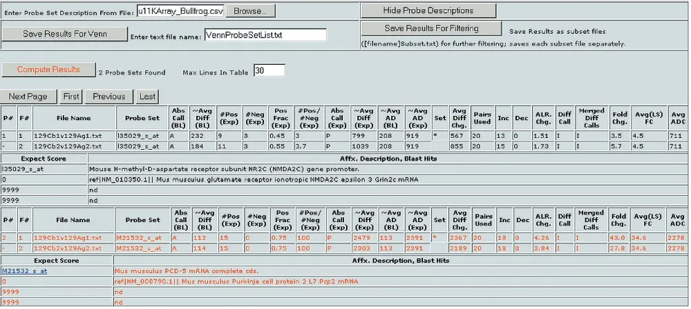
Attaching gene information

Once a filtered list of genes has been generated, gene infor-mation can be attached to the list. This inforinfor-mation can include GenBank accession numbers, UniGene numbers with direct hyperlinks to UniGene Resources, Locus Link IDs, gene names, gene descriptions, BLAST hits, protein products, functions, chromosomal locations and known associations with particular phenotypes. The gene informa-tion is stored in tables created in Microsoft Excel and must contain these columns (comma separated) in the following order: probe set or spot identifier, accession number, UniGene ID, gene title, and map location. Additional infor-mation may be added past these columns. To append gene information to a filtered list in Bullfrog or Spot, the browse button next to the ‘Enter Probe Set Description From File:’ statement at the bottom of the filter criteria table is pressed (Figure 3). The user can choose to show or hide gene infor-mation by pressing the ‘Show Probe Set Description’ button. Gene lists for the Mu11KsubA, Mu11KsubB, Hu6800, MG-U74av2, HG-U95av2 and RG-U34a Affymetrix chips are available for download as additional data files with this article or from the Barlow website [23].

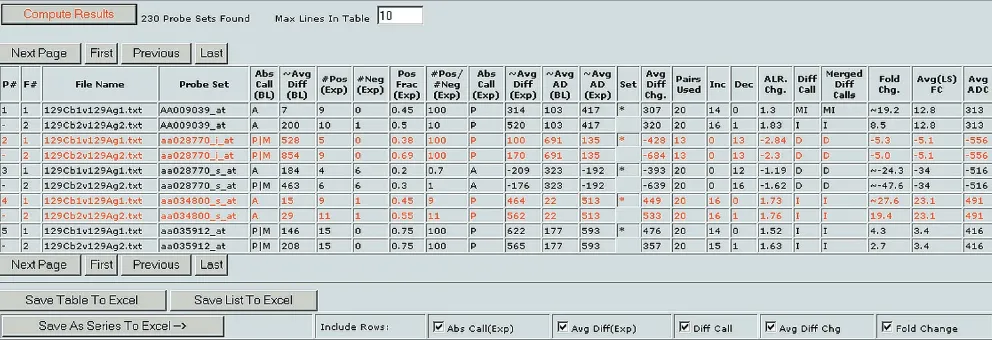
Exporting results

Genes (spots or probe sets) that pass the set filter criteria are listed in a simple table format that can be exported to Excel (Figure 4). To export the entire filtered table with all the information present, including gene information, the ‘Save Table To Excel’ button is pressed. To export a more refined list, check boxes are provided. For example, if only the fold change and average difference values are needed, the perti-nent boxes are checked and the ‘Save As Series To Excel’ button is pressed. To export a simple list of the probe sets that passed certain filter criteria, without associated infor-mation, the ‘Save List To Excel’ button is pressed. This exported data can be analyzed further in clustering and visu-alization programs. In our experience, it is often helpful to pre-filter data sets using Bullfrog and Spot before hierarchi-cal or k-means clustering [24].

Program architecture of Bullfrog and Spot

Bullfrog and Spot are Internet Explorer 5.0+ client applica-tions running on Windows NT operating systems. They are written using a combination of C++, HTML and Scripting code (VBScript and JScript). They are relatively small pro-grams, 1.1 MB and 1.2 MB respectively, and are easy to install. Double clicking the setup.bat module registers Bull-frog and Spot onto the hard drive.

comment

reviews

reports

deposited research

interactions

information

The C++ module (Atlprov.dll) performs the computationally intensive functions such as parsing and filtering the Affymetrix or cDNA data files. This module makes the data files accessible as a Microsoft OLE-DB data source, allowing script code to communicate through Microsoft’s Active Data Objects (ADO) interface. Atlprov.dll is a C++ Windows Dynamic Link Library developed with Visual Studio 6.0. The ADO Interface uses the Active Template Library (ATL) to implement the appropriate Component Object Model (COM) Interfaces, as provided by the Visual Studio Wizard for creating an OLE-DB data provider.

The Bullfrog.htm and Spot.htm modules have scripting code that uses the ADO interface to query the C++ module as if it were a database. These modules are a combination of static HTML, VBScript and JScript that produce HTML on the fly (DHTML) and use ADO commands and Recordsets. They were developed and debugged using Microsoft’s Visual InterDev and Visual Studio.NET. The static HTML provides a simple and familiar user interface for loading files and choosing filtering options. The user interface has scripts to dynamically create and modify the page’s HTML (DHTML), such as occurs when displaying a results table.

Bullfrog and Spot require that data from experiments be saved as specific file types before loading. Bullfrog requires that the data from .chp comparison files be saved as .txt files (tab-delimited text, refer to the user’s manual for complete instructions). Spot requires that data from the Excel

summary files, discussed below, be saved as .csv files (comma-separated text). These files can then be loaded into their respective programs for analysis by clicking the ‘Add Text File’ button (see Figure 2). If the ‘Prompt For File Auto Load’ box is checked, the program will automatically import up to 200 files from the same directory or folder. Once the files are loaded, clicking the ‘Complete Summary Table’ button displays relevant hybridization and data analysis information. To download the user’s manual, see the online version of this article or [23].

Features and architecture of the cDNA

normalization program

The custom cDNA normalization program is a Microsoft Excel macro and was written in Visual Basic for Applications (VBA) using Microsoft’s Visual Basic Editor. The program background subtracts and normalizes raw cDNA data before data analysis and filtering in Spot. The normalization program output includes quantitative information and quali-tative calls similar to those used for Affymetrix oligonu-cleotide arrays. Raw median pixel intensities for each gene are loaded into Microsoft Excel. Median pixel intensities are used because they are less likely to be affected by small arti-facts or slight imperfections in spot morphology. The regional background is calculated by dividing the cDNA array into 24 equal sections, and the average of the lowest 4% of spot intensities in a section is considered the section background (a section typically contains 384 to 418 spots). Figure 3

The background signal is the result of nonspecific hybridiza-tion, binding of the fluorophores to the glass surface, and fluorescence and reflection from the surface of the cDNA array. The lowest 4% of spots (typically 15-17 spots) was chosen as a balance between using multiple spots at different locations that accurately reflect nonspecific signals and not including too many spots that contain ‘real’ signals. A separate background value is calculated for each section to help correct for background that may be uneven. The background is sub-tracted from each spot in a particular section before further scaling or processing of quantitative results. For more infor-mation on background subtraction, please review the Salk cDNA analysis algorithm guide in the user’s manual folder, available with the online version of this article or at [23].

After background subtraction, the cDNA array signals are linearly scaled and normalized to compensate for non-biological variation (for example, differential fluorophore incorporation, different amounts of labeled sample, array-to-array variability). Background-subtracted signals are scaled to an overall, average target value that can be set by the user (the default value is 100). The scaling factor is cal-culated on the basis of the total signal intensity, after ignor-ing the lowest 60% and the highest 10% of signals. We determined empirically, by analyzing large amounts of cDNA array data and testing different combinations of high and low exclusion percentages, that ignoring the bottom 60% and top 10% of signals led to scaling factors that were consistent and well behaved (for example, the mean and median of the resulting distributions were approximately equal). More important, scaling factors calculated in this way consistently resulted in the smallest number of genes scoring as ‘differentially expressed’ between replicates. To

identify scaled signals that are detectable above background and to accurately estimate fold changes (ratios), a threshold is set using the scaled background values. Scaled signals that are less than the threshold are considered undetectable and are set equal to the threshold value. For more information on scaling and the setting of the thresholds please review the Salk cDNA analysis algorithm guide in the user’s manual folder, available with the online version of this article or at [23].

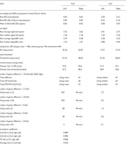
The custom cDNA normalization program generates a file in Microsoft Excel that provides a single printable summary sheet for each experiment (Table 1). The file includes infor-mation on the cDNA array background, the raw average signal intensity, the scaling factors, the thresholds, the per-centage of genes scored as present, the number of genes with fold changes (ratios) above certain thresholds and several correlation coefficients. This file provides an assessment of the overall quality of the data and a summary of the experi-mental results for each cDNA array. At the top of the summary file, not shown in Table 1, are several user-entered parameters that define the experiment. If controls were spotted on the cDNA array, a control summary is also created. In addition to the data summary, the detailed results for each spot on the microarray are provided in a table for further analysis with Spot or other programs. The results for each spot (or gene) include an absolute call of present (P) or absent (A) (a call of present indicates that the signal was greater than the regional background AND greater than the local background measured in the four corners surrounding the individual spot), the scaled intensity, the difference between the scaled fluorophore intensities, the fold change or ratio of the two-color intensities (expression

comment

reviews

reports

deposited research

interactions

information

refereed research

Figure 4

Table 1

Summary view of cDNA array data from the custom cDNA normalization program

Values Cy5 Cy3

Left Right Left Right

Raw background (BG) (using spots, lowest 4% per block)

Raw BG (mean)(spots) 0.64 0.65 2.20 2.21

Raw BG (SD of block means)(spots) 0.04 0.03 0.22 0.16

Mean of block BG SDs (spots) 0.03 0.02 0.08 0.07

Raw signal

Raw average signal (all spots) 3.73 3.65 5.01 5.57

Raw median signal (all spots) 1.24 1.18 1.94 2.10

Raw average signal/BG ratio 5.79 5.58 2.28 2.52

Raw median signal/BG ratio 1.92 1.81 0.88 0.95

Scaling factor (SF) (target value = 100), dismissing top 10% and bottom 60%

SF (using mean) 25.18 25.87 17.37 15.74

Scaled threshold

Threshold (using mean) 41.55 38.63 41.55 38.63

Percent present (using mean)

Greater than 1x BG (raw) 72.0 70.6 51.4 54.1

Greater than threshold (scaled) 47.5 48.5 48.9 50.6

Number of genes different t1.8 fold (left AND right)

Total different Using mean 43 Using median 43

Total UP (Cy5/Cy3) Using mean 20 Using median 20

Total DOWN (Cy5/Cy3) Using mean 23 Using median 23

Number of genes different t1.3 fold

Using mean (1.3) 303 Percent 7.3

Number of genes different t1.8 fold

Using mean (1.8) 204 Percent 4.5

Number of genes different t3 fold

Using mean (3) 68 Percent 1.3

Number of genes different t5 fold

Using mean (5) 28 Percent 0.6

Number of genes different t10 fold

Using mean (10) 5 Percent 0.1

Correlation coefficient

Cy5 left to Cy5 right (all) 0.989

Cy3 left to Cy3 right (all) 0.984

FC left to FC right (all) 0.968

Average Cy5 to Cy3 (all) 0.705

ratio), and a qualitative difference or change call of I, MI, D or MD (change calls are based on the fold changes across the duplicate spot data). The spot-by-spot results are easily exportable to other programs for further visualization or clus-tering. Once the cDNA data are normalized and in a system-atic format similar to the normalized Affymetrix data, the data are ready for further analysis in Spot. To download the Salk cDNA analysis algorithm guide see the user’s manual folder, available with the online version of this article or at [23].

Overall assessment

By creating an intuitive user interface with multiple, adjustable filter criteria, we have established valuable research tools for microarray users. Bullfrog, Spot and the custom cDNA normalization program were not designed to do complex statistical analyses and visualization. Rather, they were designed to help the researcher narrow their search from tens of thousands of gene candidates to several hundred or fewer that meet specific, but adjustable, criteria. Bullfrog, Spot and the custom cDNA normalization program eliminate some of the difficulty of handling large numbers of array results and allow researchers to answer crucial questions about their data quickly. These programs, along with detailed instructions and user manuals, may be downloaded at [23].

Downloading files

The microarray data analysis tools Bullfrog and Spot and associated files are available for download from the Barlow homepage [23]. Full help manuals are also available at the website.

Bullfrog and Spot analysis programs are also available for download with the online version of this article. Also available are the Bullfrog and Spot analysis programs user’s manuals, gene lists for Bullfrog, and Bullfrog and Spot sample data.

Acknowledgements

We would like to thank Lisa Wodicka, Garret Hampton, Todd A. Carter, Jo A. Del Rio, Jennifer A. Greenhall, Mario Caceres, Joel Lachuer and members of the Barlow lab for their testing and improvement suggestions. This work was supported by the H.N. and Frances C. Berger Foundation, the Lebensfeld Foundation, Charles R. Pollock, the Scher Family Founda-tion, Inc., and the Salk Institute Association. D.G.P. was supported by the Legler Benbough Fellowship.

References

1. Lockhart DJ, Winzler EA: Genomics, gene expression and DNA arrays.Nature 2000, 405:827-836.

2. Brown PO, Botstein D: Exploring the new world of the genome with DNA microarrays.Nat Genet1999, 21 (Suppl 1):33-37. 3. DeRisi J, Penland L, Brown PO, Bittner ML, Meltzer PS, Ray M, Chen

Y, Su YA, Trent JM: Use of a cDNA microarray to analyze gene expression patterns in human cancer.Nat Genet1996, 14:457-460.

4. Debouck C, Goodfellow PN: DNA microarrays in drug discov-ery and development.Nat Genet 1999, 21 (Suppl 1):48-50.

5. Coller HA, Grandori C, Tamayo P, Colbert T, Lander ES, Eisenman RN, Golub TR: Expression analysis with oligonucleotide microarrays reveals that MYC regulates genes involved in growth, cell cycle, signaling, and adhesion.Proc Natl Acad Sci USA2000, 97:3260-3265.

6. Fodor SP, Read JL, Pirrung MC, Stryer L, Lu AT, Solas D: Light-directed, spatially addressable parallel chemical synthesis.

Science1991, 251:767-773.

7. Lipshutz RJ, Fodor SP, Gingeras TR, Lockhart DJ: High density syn-thetic oligonucleotide arrays.Nat Genet1999, 21 (Suppl 1):20-24. 8. Shalon D, Smith SJ, Brown PO: A DNA microarray system for analyzing complex DNA samples using two-color fluores-cent probe hybridization. Genome Res1996, 6:639-645. 9. Hughes TR, Mao M, Jones AR, Burchard J, Marton MJ, Shannon KW,

Lefkowitz SM, Ziman M, Schelter JM, Meyer MR, et al: Expression profiling using microarrays fabricated by an ink-jet oligonu-cleotide synthesizer.Nat Biotechnol2001, 19:342-347.

10. Miles MF: Microarrays: lost in a storm of data?Nat Rev Neurosci

2001, 2:441-443.

11. Bassett DE, Eisen MB, Boguski MS: Gene expression informatics - it’s all in your mine.Nat Genet1999, 21 (Suppl 1):51-55. 12. Sandberg R, Yasuda R, Pankratz DG, Carter TA, Del Rio JA,

Wodicka L, Mayford M, Lockhart DJ, Barlow C: Regional and strain-specific gene expression mapping in the adult mouse brain. Proc Natl Acad Sci USA2000, 97:11038-11043.

13. Lockhart DJ, Barlow C: Expressing what’s on your mind: DNA arrays and the brain.Nat Rev Neurosci2001, 2:63-68.

14. Lockhart DJ, Barlow C: DNA arrays and gene expression analysis in the brain.In Methods in Genomic Neuroscience. Edited by Chin HR, Moldin SO. New York: CRC Press, 2001:143-169. 15. Lockhart DJ, Dong H, Byrne MC, Follettie MT, Gallow MV, Chee

MS, Mittmann M, Wang C, Kobayashi M, Horton H, Brown EL: Expression monitoring by hybridization to high-density oligonucleotide arrays.Nat Biotechnol1996, 14:1675-1680. 16. Wodicka L, Dong H, Mittmann M, Ho M, Lockhart DJ:

Genome-wide expression monitoring in Saccharomyces cerevisiae.Nat Biotechnol1997, 15:1359-1367.

17. Zou L, Hagen SG, Strait KA, Oppenheimer JH: Identification of thyroid hormone response elements in rodent Pcp-2, a developmentally regulated gene of cerebellar Purkinje cells.

J Biol Chem1994, 269:13346-13352.

18. Farrant M, Feldmeyer D, Takahashi T, Cull-Candy SGP: NMDA-receptor channel diversity in the developing cerebellum.

Nature1994, 368:335-339.

19. Barlow C, Hirotsune S, Paylor R, Liyanage M, Eckhaus M, Collins F, Shiloh Y, Crawley JN, Ried T, Tagle D, Wynshaw-Boris A: Atm-deficient mice: a paradigm of ataxia telangiectasia. Cell1996, 86:159-171.

20. Schena M, Shalon D, Heller R, Chai A, Brown PO, Davis RW: Paral-lel human genome analysis: microarray-based expression monitoring of 1000 genes. Proc Natl Acad Sci USA 1996, 93:10614-10619.

21. Amino-allyl dye coupling protocol

[http://derisilab.ucsf.edu/pdfs/amino-allyl-protocol.pdf]

22. Protocol for reverse transcription and amino-allyl coupling of RNA

[http://cmgm.stanford.edu/pbrown/protocols/amino-allyl.htm] 23. Carolee Barlow [http://www.salk.edu/faculty/barlow.html] 24. Carter TA, Del Rio JA, Greenhall JA, Latronica ML, Lockhart DJ,

Barlow C: Chipping away at complex behavior: transcrip-tome/phenotype correlations in the mouse brain. Physiol Behav2001, 73:849-857.