Multi-objective optimisation of machine tool error mapping using
automated planning
S. Parkinson
a,⇑, A.P. Longstaff
b aDepartment of Informatics, School of Computing and Engineering, University of Huddersfield, Queensgate, Huddersfield HD1 3DH, UK b
Centre for Precision Technologies, School of Computing and Engineering, University of Huddersfield, Queensgate, Huddersfield HD1 3DH, UK
a r t i c l e
i n f o
Article history:
Available online 9 December 2014
Keywords:
Machine tool error mapping Uncertainty of measurement Automated planning PDDL
Multi-objective optimisation
a b s t r a c t
Error mapping of machine tools is a multi-measurement task that is planned based on expert knowledge. There are no intelligent tools aiding the production of optimal measurement plans. In previous work, a method of intelligently constructing measurement plans demonstrated that it is feasible to optimise the plans either to reduce machine tool downtime or the estimated uncertainty of measurement due to the plan schedule. However, production scheduling and a continuously changing environment can impose conflicting constraints on downtime and the uncertainty of measurement. In this paper, the use of the produced measurement model to minimise machine tool downtime, the uncertainty of mea-surement and the arithmetic mean of both is investigated and discussed through the use of twelve dif-ferent error mapping instances. The multi-objective search plans on average have a 3% reduction in the time metric when compared to the downtime of the uncertainty optimised plan and a 23% improve-ment in estimated uncertainty of measureimprove-ment metric when compared to the uncertainty of the tempo-rally optimised plan. Further experiments on a High Performance Computing (HPC) architecture demonstrated that there is on average a 3% improvement in optimality when compared with the exper-iments performed on the PC architecture. This demonstrates that even though a 4% improvement is ben-eficial, in most applications a standard PC architecture will result in valid error mapping plan. Ó2014 The Authors. Published by Elsevier Ltd. This is an open access article under the CC BY license (http://
creativecommons.org/licenses/by/3.0/).
1. Introduction
A machine tool is a mechanically powered device used during subtractive manufacturing to cut material. The design and config-uration of a machine tool is chosen for a particular role and is dif-ferent depending, amongst other things, on the volume and complexity range of the work-pieces to be produced. A common factor throughout all configurations of machine tools is that they provide the mechanism to support and manoeuvre the functional position, and sometimes the orientation, between the cutting tool and work-piece. The physical manner by which the machine moves is determined by the machine’s kinematic chain (Moriwaki, 2008). The kinematic chain will typically constitute a combination of lin-ear and rotary axes.
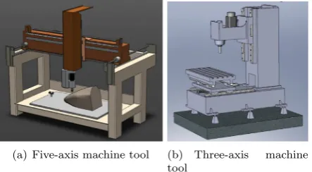
Fig. 1(a) shows an example of a five-axis gantry machine tool that has three linear and two rotary axes which are used to move the tool around the work-piece. Typically, this configuration of machine will be used to machine heavy, multi-sided, large volume
work-pieces.Fig. 1(b) shows an alternative design of a three-axis C-frame machine tool. This particular machine tool configuration consists of three linear and no rotary axes and is typically used to machine smaller work-pieces than the five-axis machine.
In a perfect world, a machine tool would be able to move to pre-dicable points and orientations in three-dimensional space, result-ing in a machined artefact that is geometrically identical to the designed part. However, due to tolerances in the production of machine tools and wear during operation, this is very difficult to achieve mechanically. Pseudo-static errors are the geometric posi-tioning errors resulting from the movement of the machine tool’s axes that exist when the machine tool is nominally stationary. Machine tool error mapping is the process of quantifying these errors (Schwenke et al., 2008) so that predictions as well as improvements of part accuracy can be made via numerical analysis and compensation.
The significance of the error mapping process is dependent on application; manufacturers machining high value parts to tight tol-erances, usually in the order of less than a few tens of micrometres, should have their machines regularly error mapped otherwise they are at risk of producing non-confirming parts. Manufactures with broader tolerances may calibrate less frequently. There are many
http://dx.doi.org/10.1016/j.eswa.2014.11.066
0957-4174/Ó2014 The Authors. Published by Elsevier Ltd.
This is an open access article under the CC BY license (http://creativecommons.org/licenses/by/3.0/).
⇑ Corresponding author.
E-mail addresses:[email protected](S. Parkinson),[email protected] (A.P. Longstaff).
Contents lists available atScienceDirect
Expert Systems with Applications
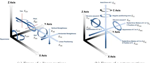
error components that collectively result in deviation of the machine tool from the nominal. For analytical and correction pur-poses, it is important to measure each error component. For exam-ple, as seen inFig. 2(a) a machine tool with three linear axes will have twenty-one geometric errors. This is because each linear axis will have six-degrees-of-freedom and a squareness error with the nominally perpendicular axes (Mekid, 2009; Schwenke et al., 2008). Therefore, a three-axis machine tool will have a total of twenty-one geometric errors. Additionally, as seen inFig. 2(b) a rotary axis will have six motion, two location errors, and two squareness errors (Bohez et al., 2007; Khim and Keong, 2010; Srivastava et al., 1995). Therefore, a five-axis machine tool will have a total of forty-one geometric errors.
The measurement of each error will involve the use of a test method and a measurement device. The selection of equipment will usually be done in unison with the test method, influenced by the engineer’s preference. However, there are many cases where many different instruments can be used for performing the same test method, where each require a different duration to install and perform the test. For example, both a laser interferometer and a granite straight edge can be used to measure the straightness of a linear axis. The laser interferometer might take longer to set-up, but if the machine has an axis with a long travel, the granite straight edge might need to be repositioned multiple times to mea-sure the entire axis, therefore, taking more time to perform. For most manufacturers, removing a machine tool from manufacturing has large financial implications. Downtime can be in excess of £120 per hour (Shagluf et al., 2013). Therefore, the accumulative cost for a manufacturer with many machines can be large. For example, consider a manufacturer with 10 machine tools, each of which undergoes a 12 h error mapping exercise per year. The estimated downtime cost would be £14,400. However, this is a conservative figure for many high value manufacturing companies.
The estimated uncertainty of measurement is a parameter asso-ciated with the result of a measurement that characterises the dis-persion of the values that could reasonable be attributed to the measurand (BIPM, 2008). The uncertainty of measurement is cal-culated for each individual measurement and the accumulative estimated uncertainty of measurement has a direct effect on toler-ance conformtoler-ance of parts manufactured using the machine. Therefore, from the manufacturer’s perspective, it is desirable to reduce the estimated uncertainty of measurement. The estimated uncertainty of measurement is affected by change in environmen-tal temperature. If the same calibration plan was carried out at dif-ferent times throughout a working-day while the temperature is continuously changing, the accumulative estimated uncertainty would also change.
Depending upon the manufacturer’s motivation for performing the error map, they may want to optimise the error map plan to either minimise financial cost, or maximise the quality of the error mapping exercise. The following different optimisation criteria
considered in this paper are: (1) the reduction of machine tool downtime, (2) the reduction of the estimated uncertainty of mea-surements, and (3) balancing the two parameters with the possi-bility of customising their individual weighting. The change in environmental temperature throughout a measurement, as well as between interrelated measurements, will have a significant impact on estimated uncertainty of measurement ISO230-9 (2005). The decision making process involved for construction optimal error maps plans is exhaustive. However, computational intelligence in the form of domain-independent Artificial Intelli-gence (AI) can be used to provide optimal solutions when given a model of the problem (Ghallab et al., 2004).
In this paper, a description of individual factors that affect a machine’s downtime and estimated uncertainty of measurement during error mapping are defined. This leads to a discussion of a previously developed model (Parkinson et al., 2012a, 2012b) that can be used by state-of-the-art domain-independent AI planning tools to find optimised solutions (Russell et al., 1995). The develop-ment of this model to produce measuredevelop-ment plans that are opti-mised to reduce machine downtime and the estimated uncertainty of measurement due to the plan order is presented and discussed. This multi-objective optimisation is motivated by the desire to reduce both machine tool downtime and the uncer-tainty of measurement, which to some extent are competing as a temporally optimised plan will generally have a high estimated uncertainty of measurement. Following the development of a multi-objective model, twelve different case-study examples are presented and described to show the ability to generate plans that are optimised for (1) downtime, (2) uncertainty of measurement, and (3) the arithmetic mean of them both. The generated calibra-tion plans are then examined and discussed to evaluate their fit-ness-for-purpose. It is then identified that computational resources are restricting the planner’s ability to find optimal solu-tions in ten minute time allocation. This leads to a further investi-gation into the produced measurement plan when solving the planning problem on both personal and High Performance Com-puting architectures.
2. Related work
The complexity associated with machine tool geometric error measurement (Mekid, 2009; Schwenke et al., 2008) and the desire to reduce measurement uncertainty (Bringmann and Knapp, 2009;
Bringmann et al., 2008) and machine tool downtime are well
known for individual measurements. However, surveying the liter-ature suggests that less well known is the potential to reduce machine tool downtime and the uncertainty of measurement by intelligent construction of the multiple-measurement plan.
Bringmann and Knapp (2009) and Bringmann et al. (2008)have identified that current ISO 230 part 2 (ISO230, 2006) is based on sequential testing of single geometric component errors. However, an exception is made for ISO 230 part 4 (ISO230, 2005) where sev-eral machine errors are tested together while the machine tool is performing multi-axis movement.Bringmann and Knapp (2009)
then continue to describe the importance of interrelated errors using the example of linear yaw deviation effecting the non-orthogonality measurement at different positions in the plane of non-orthogonality measurement. The authors identify that this process is time consuming, and in response have shown the cali-bration of a machine tool using a 3D-ball plate where the amplifi-cation of interrelated measurements can be identified. However, when such approach cannot be used, they suggest using a Monte Carlo simulation that uses an approximation of the machine tool, the measurement and the machine’s performance after calibration to estimate the uncertainty of measurement. Performing the (a) Five-axis machine tool (b) Three-axis machine
[image:2.595.49.271.615.737.2]tool
Monte Carlo simulation sufficiently often will produce a distribu-tion for the uncertainty of the identified errors. This work suc-ceeded in producing optimal measurement plans when considering interrelated measurements by suggesting the use of a 3D-ball plate, or measurement uncertainty of measurement reduction using Monte Carlo simulation. In one example, the uncertainty of measurement for the X-axis linear positioning error EXXis reduced from 30
l
m to 10l
m. The limitation of this work isthat it is concerned with achieving the best possible measurement sequence with respect to the uncertainty of measurement at all costs, ignoring machine tool downtime.
Muelaner et al. (2010) produced a method of large volume
instrumentation selection and measurability analysis. This work is not explicitly for machine tool calibration, but does considers the suitability of instrumentation based on measurement method and instrumentation criteria. This implementation results in a pro-totype piece of software capable of finding the best instrumenta-tion and measurement method from an internal database. Although this work is capable of always finding the optimum selec-tion based on the predefined criteria, it pays no consideraselec-tion to temporal aspects. Additionally, the produced model and software does not take any consideration to interrelated measurements, allowing for optimal sequencing.
Recent advancements in measurement instrumentation have demonstrated how multiple error components can be measured simultaneously using the same instrument. These techniques can simplify the calibration planning process as the calibration will require less time to complete, making the duration between mea-surements lower. Therefore, the likelihood of being able to sche-dule the measurements to happen over a duration that is temperature-stable is increased. However, this significantly depends on the machine tool’s environment. For example, the API XD™ (API, 2014) allows for measuring all 6DOF simultaneously for one linear horizontal axis from a single set-up.
Other methods of machine tool calibration include being able to measure indirectly all the geometric error components simulta-neously. One such method is the Etalon laserTRACER (Etalon, 2014) which has a linear measurement resolution of 0.001
l
m for measuring axes up to 15 m in length. The laserTracer tracks the actual path of the machine tool throughout the entire working volume. This is done by attaching a reflector on the machine tool at the tool fixing point. From the acquired information, the system can perform a full calibration of multiple axis Cartesian machines. This includes all six-degrees-of-freedom and the non-orthogonal error. Using this method to calibrate a machine tool reduce the requirement for the use of multiple instrumentation and measure-ment methods, therefore, the type of calibration planning dis-cussed in this thesis is reduced. However, due to the expensive cost of such equipment, the majority of machine tool owners and providers of calibration services will not yet own such a device.The literature survey suggests that although both industrial and academic experts are currently producing valid machine tool cali-bration plans, there is little evidence to suggest that they are con-sidering optimisation. It has also been identified that there is a desire to minimise machine tool downtime during calibration and to improve the machine’s accuracy. From these observations, it has been established that there is potential benefit from develop-ing a method to automatically produce optimised machine tool cal-ibration plans.
3. Perspectives of optimisation
3.1. Temporal optimisation
A machine tool will not be available for normal manufacturing while the error mapping process is taking place. For this reason, it is important to consider the temporal aspects when performing a measurement. Measuring an error component has several tempo-ral implications (Schwenke et al., 2008). The following list describes the different phases associated with all measurements. The duration of each phase is based on empirical observation (Parkinson et al., 2012a) and can easily be adjusted should the user require.
1. Set-up of the instrumentation is normally a manual process where the instrumentation will be taken from its protective packaging and set-up on the machine for use. This duration includes time taken for fine tuning of the instrumentation (e.g laser beam alignment) and it can also include the time taken for the instrument to stabilise in terms of self-heating and sta-bilising to the environmental conditions, although with good planning this can be achieved ‘‘offline’’ without the need for the machine.
2. Measurement of the component error can be manual or automated, but either way it will still require time to complete. During measurement, the measurement data as well as any necessary environmental data will be recorded. The duration will be affected by the sampling frequency, interval between targets, dwell time to take a measurement, and the feedrate of the machine.
[image:3.595.147.458.65.197.2]3. Removal, adjustment and repositionof instrumentation are post-measurement durations. Removal is simply the time taken to remove the instrumentation and package it suitable for stor-age. Adjustment is the duration for when an instrumentation is required to be adjusted to measure another component error. For example, after measuring linear positioning using a laser interferometer the optics could be changed to angular optics without having to go through the complete set-up. Reposition-ing is where the instrument needs movReposition-ing to perform another measurement for the same component error. For example, (a) Errors of a linear motions (b) Errors of a rotary motions
when measuring straightness of a long axis using a Short Range Displacement Transducer (SRDT) and a granite straight edge it is possible that the straight edge will need to be repositioned multiple times to cover a sufficient amount of travel. Another example is using a granite square and SRDT; the square can be adjusted to measure another axis, taking less time than set-ting the instrumentation up in the first instance. In this analysis, the ‘‘taking out of the box’’ is not included. It is assumed that the measurement engineers have expertise to do this efficiently. However, planning could be extended to include this.
3.1.1. Downtime calculation
During planning, the estimated machine tool downtime can be calculated by summing the individual durations associated with each measurement. A minimisation function can be used return the most efficient selection of measurements where the objective is to reduce estimated time. Each measurement task is comprised of several sub-tasks that have an associated duration.
fðtÞ ¼min X n
i¼1
m X
n
i¼1 d
!!
ð1Þ
Eq.(1)shows an abstract minimisation function,fðeÞ, for measuring the machine tool t, wherem are individual measurements (error component) and is made up of the sum of durations,d. For example, the duration to setup a measurement and the duration to perform the measurement.min is the combination ofdfor measurement mwhere the accumulation of all the durations is as low as possible.
3.2. Uncertainty of measurement
Uncertainty of measurement is a parameter associated with the result of a measurement that characterises the dispersion of the values that could reasonable be attributed to the measurand (BIPM, 2008). For example, a thermometer might have an uncer-tainty value of ±0.1°C. Therefore, it can be stated that when the thermometer is displaying 20°C, it is actually 20°C ±0.1°C with a confidence level of 95% where the confidence level is determined by the distribution and knowledge of the system. Quantifying and reducing uncertainty of measurement is an important task and is required to be reported on the calibration certificate. More impor-tantly, it is required to determine if the measurement method is suitable to establish whether the machine is capable of meeting its tolerances.
The philosophy behind the investigation performed in this paper is that, rather than calculating the total estimated
uncertainty for each individual measurement, it is more efficient to consider only the contributors due to scheduling that affect the estimated uncertainty. This means that it is only necessary to model aspects that cause the estimated uncertainty of measure-ment to change, thus simplifying the domain model.
There are many potential contributors that affect the uncer-tainty of measurement. However, when automatically constructing an error map plan, the aim is to select the most suitable instrumen-tation and measurement technique that has the lowest estimated uncertainty. In addition, the estimated uncertainty should take into considering the changing environmental data, and where pos-sible, schedule the measurements to take place where the effect of temperature on the estimated uncertainty is at its lowest.
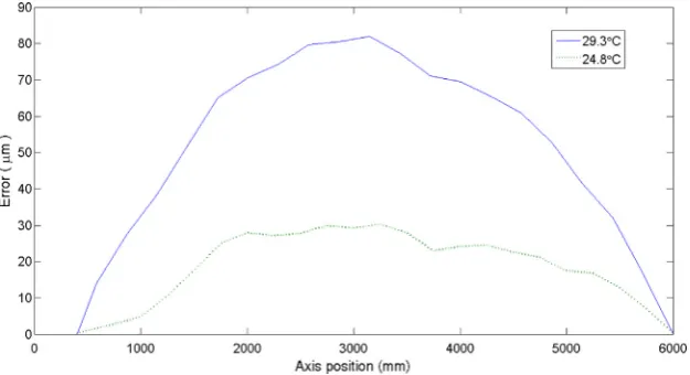
Fig. 3shows a real-world example of the Y-axis straightness in the X-axis direction measured on a gantry milling machine at two different temperatures. From this figure, it is evident that the error quadruples with a 4.5°C increase in temperature. This example illustrates the different of measuring the same error component at different temperatures and motivates the significance that envi-ronmental temperature has on the estimated uncertainty of measurement.
The following list provides the factors that affect the estimated uncertainty of the error map plan, and suggests how they can be optimised.
Measurement instrumentation having the lowest estimated uncertainty of measurement. Where possible, intelligently selecting instrumentation with the lowest uncertainty will reduce the overall estimated uncertainty of measurement. However, they may also have a higher temporal cost.
The change in environmental temperature throughout the dura-tion of a measurement can significantly increase the uncer-tainty of measurement. When possible, the measurement should be scheduled to take place where the temperature is stable.
When considering inter-related measurements, the change in environmental temperature between their measurement can significantly increase the uncertainty. During planning, it is important to schedule interrelated measurements where the change in environmental temperature is at its lowest. For exam-ple,Mian et al. (2013)report a 5°C environmental temperature change over a three day period that resulted in 18
l
m displace-ment in the Y-axis and 35l
m in the Z-axis. [image:4.595.138.451.569.739.2]Allowing the instrument to correctly stabilise in the environ-ment before the measureenviron-ment can reduce the uncertainty due to thermal distortion and self-heating.
3.2.1. Uncertainty calculation
One known method, recommended by International Standards Organisation (ISO), involves combining the individual uncertain-ties using the root of the sum of squares to produce a combined uncertainty uc. In this paper, Eq. (2) is used for calculating uc
(ISO230-9, 2005; BIPM, 2008).
uc¼
ffiffiffiffiffiffiffiffiffiffiffiffiffi X
u2 i
q
ð2Þ
Where uc is the combined standard uncertainty in micrometers
(
l
m), anduiis the standard uncertainty of uncorrelated contributor,i, in micrometers (
l
m).Onceuchas been calculated, the expanded uncertainty is
calcu-lated by multiplying uncertaintyUcby the coverage factork, which
in this case isk¼2 which provides a confidence level of 95%. A comprehensive example of calculating the uncertainty of measurement for measuring the squareness of two perpendicular axes can be found inParkinson et al. (2014a, 2014b).
4. Automated planning
Planning is an abstract, explicit deliberation process that chooses and organises actions by anticipating their expected out-come. Automated planning is a branch of Artificial Intelligence (AI) that studies this deliberation process computationally and aims to provide tools that can be used to solve real-world planning problems (Ghallab et al., 2004).
Domain-independent planning is a form of planning where a piece of software (planner) takes as input the problem specifica-tion and knowledge about the domain in the form of an abstract model of actions. Searching for solution plans is a PSPACE hard problem (Erol et al., 1995). PSPACE describes the computational complexity associated with decision problems that can be solved by a Turing machine using a polynomial amount of space. One key difficulty encountered with domain-independent planners is the very broad range of planning problems which could be presented, requiring any guidance strategy to be effective across the potential range of problems.
Advances in domain-independent research resulted in the for-mation of the International Planning Competition (IPC) (McDermott, 2000) where state-of-the-art planners try to solve an ever increasing set of complex benchmark problems. The birth of the IPC brought a standardised formalism for describing plan-ning domains and problems that could be used to make direct comparisons between the performance of planners. Therefore, sup-porting faster progress in the community. This formalism is called the Planning Domain Definition Language (PDDL) (McDermott et al., 1998) and has gone through many revisions where new fea-tures, allowing for more expressive domain modelling, have been added.
5. Domain model
The previously developed temporal model (Parkinson et al.,
2012a, 2012b) has been extended to encode the knowledge of
uncertainty of measurement reduction (Parkinson et al., 2014a).
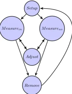
Fig. 4shows the functional flow between the PDDL actions within the extended model. In the figure, durative actions are represented using a circle with a solid line.Fig. 4shows that the measurement action has been split up into two different action and an adjust action has been added which may need to be executed if the instrumentation is not effective for the travel length of the axis. It is necessary to have two versions of the measurement action because not all measurements have other errors propagating down the kinematic chain and effecting their uncertainty. The following
list details the extension of the measurement action into two actions along with and adjustment action:
Measureno: The measurement action represents a measurement
where no consideration is required to be taken for any inter-related measurements.
Measurein: Conversely, this measurement action represents a
measurement where consideration is required to be taken because of inter-related measurements. Adjust: Some axes are longer than the range of the
measur-ing device. In this case, the measurmeasur-ing device needs to be readjusted, perhaps several times, in order to measure the full range of the axis.
The developed model is encoded in PDDL 2.1 because it uses numbers, time, and durative actions (Fox and Long, 2003). Regular numeric fluents to model constants and variables relating to the uncertainty of measurements. For example, a device’s uncertainty (UDEVICE LASER) can be represented in PDDL as (=(deviceu?i
-instrument) 0.001) where the instrument object ?i has the value of 0.001
l
m.In the temporal model, the cost of each action is the time taken to perform that specific task. Using this model will produce an error map plan, indicating the ordering of the measurements and the time taken to perform each test. In order to encode tempera-ture dependent equations, access is needed to the change in envi-ronmental temperature that occurs between the start and end of a measurement. Assuming access to the temperature as a fluent, the value can be sampled at the start and end of the measurement with theat startandat endsyntax of PDDL. Thus, a temporary value (start-temp) is recorded at the start of the action, and then cal-culateTDat the end of the action by subtracting the start temper-ature from the current tempertemper-ature.
As stated previously, in order for this modelling choice to work, it must be possible to query the temperature as a fluent at any given time. The method used in order to achieve this is described in the following section.
5.0.2. Temperature profile
In PDDL2.1 it is not possible simply to represent predictable continuous, non-linear numeric change. More specifically, it is not possible to represent the continuous temperature change throughout the error mapping process. This presents the challenge of how to optimise the sequence of measurements while consider-ing temperature. The solution implemented in the model involves
Setup
M easurein M easureno
Adjust
[image:5.595.374.500.67.232.2]Remove
discretizing the continuous temperature change into sub-profiles of linear continuous change.
This environmental temperature profile contains the systematic heating and cooling profile for the environment of a machine tool. This information can be obtained by non-invasive monitoring or historical date from the machine tool owner. It is not possible to predict the non-systematic environmental temperature deviation and the magnitude of the systematic element could fluctuate slightly. However, using this systematic profile will allow us to pre-dict how the temperature will change throughout the day, in par-ticular where the rate of change is at its lowest. Scheduling against this profile gives the best available chance of producing realistic and accurate results. During the actual error mapping process, deviations from the systematic profile are recorded and taken into account on the calibration certificate.
The continuous temperature profiles are split up into a discrete set of linear sections by iterating over the temperature data looking for a difference in temperature greater than a given sensitivity. This allows the temperature profile to be discretized into a set of linear sub-profiles. An example can be seen in Fig. 5where the environmental temperature profile (difference from 20°C) for a forty-eight hour period is shown (Monday and Tuesday). The cho-sen cho-sensitivity,s, is based on the minimum temperature sensitivity of the available instrumentation. In this example, it is 0.1°C. The graph shows the temperature profile across 48 h; the second 24 h period displays a higher temperature profile than the first and appears to reach relative stability. The reason is due to the ini-tial state on the Monday morning after the weekend shut-down.
To model these sub-profiles in the PDDL model, they are repre-sented as predetermined exogenous effects. In order to encode these in PDDL2.1, the standard technique of clipping durative actions together is used (Fox et al., 2004). The#tsyntax is used to model the continuous linear change through the subprofile. Because the (temp) fluent is never used as a precondition, the measure actions can make use of the continuously changing value, without violating theno moving targets(Long and Fox, 2003) rule. Given the predefined timest1;. . .;tnwhen the sub-profilep1;. . .:pn
will change, a collection of durative actions,d1;. . .dnare created
that will occur for the durationst1;t2t1;. . .;tntn1. An example
durative actiond1that represents a sub-profilep1can be seen in
Fig. 6 where the duration t1¼42. In the measure-influence
action, the temperature at the start of the measurement action, t1, and at the end of the action,t2are stored instart-tempand temp, respectively. Therefore, in the measurement action it is pos-sible to calculate the maximum temperature deviation,DT, based on two temperatures,t1andt2.
5.0.3. Uncertainty equations
Implementing equations where the result is influenced by other measurements is also encoded in the PDDL using numeric fluents. For example,Fig. 7shows the calculation for the squareness error measurement using a granite square and a dial test indicator where the uncertainty is influenced by the two straightness errors. In the model, this is encoded by assigning two fluents (error-val?ax?e1))and(error-val?ax?e2)), the maximum permis-sible straightness error in the PDDL initial state description. This fluent will then be updated once the measurement estimation has been performed. The planner will then schedule the measure-ments to reduce the effect from the contributing uncertainty. This shows how the uncertainty can be reduced due to the ordering of the plan.
5.1. Planner
Local Search for Planning Graphs with Timed Initial Literals (TILs) and derived predicates (LPG-td) (Gerevini et al., 2008) is a domain-independent planning tool and was a top performer in the third International Planning Competition (IPC) (Long and Fox, 2003), solving 428 planning problems with a success of 87%. Addi-tionally LPG-td was a top performer involving domains with pre-dictable exogenous events (which are TILs in PDDL) (Gerevini et al., 2006). LPG-td implements an extended local search algo-rithm and action graph representation. This representation is a Numerical Action (NA) graph which extends the action graph (Gerevini and Serina, 2002) to contain propositional nodes and numerical nodes, labelled with propositions and numerical expres-sions, respectively (Serina, 2004). Since the production of LPG-td, many other planners have been developed that can solve PDDL2.2 problems and beyond. However, there are few planners that can support the full semantics of PDDL.
6. Experimental analysis
To examine the relationship between optimisation of temporal and the uncertainty of measurement, twelve different PDDL prob-lem instances are used and optimised for following three different metrics:
1. U–(:metric minimize (u-m)) 2. T–(:metric minimize (total-time)) 3. ðUþTÞ
2 –(:metric minimize (/(+(u_c)(totaltime))2))
The notation of problem instances used within this paper repre-sents the configuration of the machine tool (3 and 5 axis), the range of available instrumentation (1 or 2), and the experience of
(:durative-action temp-profile1
:duration(= ?duration 42.0)
:condition
(and(over all(not(start0)))
(over all (start1))))
:effect
(and
(rate)0.00595))
(increase (temp)(*#t 0.00595))
(at end (not(start1)))
(at end (start2))
[image:6.595.321.520.68.205.2](at start (clip-started))))
)
Fig. 6.Durative actions that represents the temperature sub-profilep1where the duration ist1¼42.
0 10 20 30 40 50
0 2 4
Time in Hours
T
emp
erature
difference
from
20
◦C
Measured Temperature Discretized Temperature
[image:6.595.66.253.570.729.2]the measurement engineer (1, 2, and 3). For example, problem instance 32A represents a three-axis machine tool with the potential use of a wide range of instrumentation planned by a measurement engineer with limited experience.
[image:7.595.44.295.615.753.2]The experiments were performed on an AMD Phenom II 3.50 GHZ processor with 4 GB of RAM. The results show the most efficient plan produced within a 10 min CPU time limit. All the pro-duced plans are then validated using VAL (Howey et al., 2004). VAL is the automatic validation tool for PDDL that is capable of validat-ing PDDL solutions against PDDL problems and domains. These experiments were carried out without the ability to schedule mea-surements concurrently. This is because in this current model, the effect that concurrent measurements will have on the uncertainty of measurement has not been accounted for. It is likely that uncer-tainties could improve due to lower change in ambient conditions during relative measurements, but this could be counteracted by any need to use instrumentation with a higher uncertainty in order to achieve concurrent measurement.
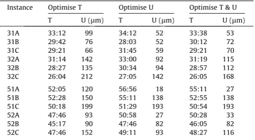
Table 1shows the empirical data from performing these exper-iments. From these results, it is evident that when optimising for time, no consideration is taken for the uncertainty due to the plan order. Similarly, it is evident that when optimising for the uncer-tainty due to the plan order, no consideration for temporal impli-cations is taken. However, when optimising the plan for both the
uncertainty due to the order of the plan and reducing the overall timespan, it is evident that the planner can establish a good compromise.
FromTable 1it is noticeable that a solution to each problem instance is found within the 10 min time limit. In addition,Table 2 shows exactly how many plans were produced during this time-limit and at what time the optimal plan was discovered. This information shows that the optimal plans were discovered on aver-age after 8 min 29 s of execution. This highlights that it is possible that the optimal plans are not being found within the 10 min per-iod. It is also worth highlighting that the results demonstrate the potential advantage of using automated planning based on the developed model. However, it is possible that experts with differ-ent opinions and knowledge might produce error map plans that have a lower estimated uncertainty of measurement. Encoding this new knowledge in the model would then allow for comparable optimised error map plans to be produced.
6.0.1. High Performance Computing
To investigate this further, without imposing a strict computa-tion restriccomputa-tion, experiments were performed on a hardware platform with increased resource availability. The chosen platform is the Huddersfield University QueensGate Grid (QGG) High
Table 1
Temporal & uncertainty optimisation results (PC) (hours:minutes).
Instance Optimise T Optimise U Optimise T & U
T U (lm) T U (lm) T U (lm)
31A 33:12 99 34:12 52 33:38 53
31B 29:42 76 28:03 52 30:12 72
31C 29:21 66 31:45 59 29:21 70
32A 31:14 142 33:00 92 31:19 115 32B 28:27 135 30:34 94 28:57 112 32C 26:04 212 27:05 142 26:05 168
51A 52:05 120 56:56 18 55:11 27 51B 52:28 150 55:11 138 52:55 138 51C 50:18 199 51:29 193 50:54 193
52A 47:46 93 50:58 27 50:28 33
52B 45:17 90 47:46 82 46:05 82
[image:7.595.310.562.616.754.2]52C 47:46 152 49:11 93 48:27 116
Table 2
The number of identified plans and the discovery time of the optimal (minutes:seconds).
Instance Optimise T Optimise U Optimise T & U
# T # T # T
31A 6 8:58 1 7:48 6 9:43
31B 5 7:45 1 9:21 5 9:02
31C 6 5:10 2 8:08 3 7:26
32A 8 9:20 2 8:40 4 8:40
32B 5 8:42 2 9:26 5 9:08
32C 7 9:47 1 7:14 2 8:19
51A 3 9:55 1 8:37 3 9:37
51B 2 9:36 1 8:33 1 9:50
51C 3 8:23 1 8:48 4 8:09
52A 4 7:39 2 9:20 5 9:41
52B 2 5:42 2 7:25 2 7.01
52C 4 9:00 2 8:08 1 7:51
(at start(assign(temp-u)
;calculate u device using the length to measure.
(+(*(/(k value ?in)(*(u calib ?in)(length-to-measure ?ax ?er)))
(/(k value ?in)(*(u calib ?in)(length-to-measure ?ax ?er))))
;calculate u misalignment.
(+(*(/(+(u misalignment ?in)(u misalignment ?in))(2sqr3))
(/(+(u misalignment ?in)(u misalignment ?in))(2sqr3)))
;calculate u error contributors.
(+(*(/(+(error-val ?ax ?e1)(error-val ?ax ?e2))(2sqr3))
(/(+(error-val ?ax ?e1)(error-val ?ax ?e2))(2sqr3)))
;calculate u m machine tool.
(+(*(*(u t-m-d)(*(length-to-measure ?ax ?er)(u m-d)))
(*(u t-m-d)(*(length-to-measure ?ax ?er)(u m-d))))
;calculate u m device.
(+(*(*(u t-m-d)(*(length-to-measure ?ax ?er)(u m-d)))
(*(u t-m-d)(*(length-to-measure ?ax ?er)(u m-d))))
;calculate u eve.
(*(/(u eve)(2sqr3))(/(u eve)(2sqr3))))))))
)
)
Performance Computing (HPC) architecture. The dedicated hard-ware has 37 cores with a clock speed of 2.53 GHz with an allocated 8 GB of RAM to each core. The same experiments as for the PC were performed on the QGG with a CPU execution time-limit of 24 h. The motivation behind allowing the planners to run for 24 h is because the HPC architecture has clock speeds comparable with a PC architecture. As LPG-td is a single-core application, allowing the planner to execute for only 10 min would yield similar results as on the PC. Therefore, the chosen HPC architecture creates the possibility to execute many instances of LPG-td simultaneously and for prolonged periods which would render the average PC unusable for other activities.Table 3shows the results from these experiments. From these results, it is evident that in almost all instances plans have been found with a lower metric. This highlights that providing significantly more computation time can result in plans that are better optimised. However, it is impor-tant to consider the gain in optimality to evaluate whether the extra computational resources are necessary. Table 4 shows the percentage improvement for each metric when comparing the experiments performed on the QGG and those on the PC. It is noticeable that while in most cases there is an improvement in the optimised metric, there is also often deterioration for the non-optimised metric. Additionally, there is an improvement for both metrics for the multi-object experiments.
The use of the QQG has shown that improvements over the optimal solutions identified on a PC can be achieved by using greater computation power. However, determining whether this is necessary is down to the end user. For example, for a measure-ment engineer wishing to perform a quick and effective error mapping process on an old machine tool operating with large
tolerances, the use of a PC architecture is sufficient. Conversely, a measurement engineering error mapping a state-of-the-art machine tool that operates to sub-micron tolerances within the aerospace sector will want to perform both the quickest and most effective error mapping plan that can minimise the uncertainty of measurement, making the use of HPC for this engineer is justified.
6.1. Plan excerpts
The following three plan excerpts (Figs. 8–10) illustrate the pro-duced plans for the three different metrics and the differences between the order of measurement.
[image:8.595.331.527.292.504.2]Fig. 8shows an excerpt from a temporally optimised plan pro-duced from the 31A problem instance. The motivation for showing this particular excerpt is to investigate how the measurement of interrelated errors is scheduled in the produced plan. Firstly, it is noticeable in the plan that the measurements that can use the same instrumentation are clustered together so the instruments can be adjusted from a previous measurement to save time, rather
Table 3
Temporal & uncertainty optimisation results (Cluster) (hours:minutes).
Instance Optimise T Optimise U Optimise T & U
T U (lm) T U (lm) T U (lm)
31A 32:42 137 34:32 52 32:52 18 31B 29:14 197 31:45 49 29:34 138 31C 29:15 80 31:57 67 29:15 193 32A 30:52 142 32:50 90 31:03 27 32B 28:12 135 29:27 89 28:57 82 32C 25:56 293 26:41 139 26:05 93
[image:8.595.32.285.422.561.2]51A 51:52 137 63:20 18 52:50 52 51B 51:00 271 57:17 138 52:35 63 51C 49:05 291 53:38 193 50:11 67 52A 47:46 114 49:44 27 47:46 95 52B 45:02 89 47:46 82 45:52 112 52C 47:22 162 48:32 88 47:46 114
Table 4
Percentage improvement between QQG and PC (hours:minutes).
Instance Optimise T Optimise U Optimise T & U
T (%) U (%) T (%) U (%) T (%) U (%)
31A 1 21 1 0 2 2
31B 2 62 2 13 2 14
31C 0 17 1 12 0 5
32A 1 0 0 2 1 21
32B 1 0 4 7 0 0
32C 0 28 1 2 0 19
51A 0 13 10 0 4 50
51B 3 45 4 0 1 0
51C 2 32 4 0 1 0
52A 0 19 2 0 6 20
52B 1 1 0 0 1 0
52C 1 6 1 5 1.4 25
Average 1 21 1 1 2 13
Instrumentation set-up Instrumentation adjustment Measurement
Set-up removal
EXY: Straightness of the Y-axis in the X-axis direction
EZY: Straightness of the Y-axis in the Z-axis direction ECY: Angular deviation around the C-axis
EC0Y: Non-orthogonality between the Y- and X-axis
EB0Z: Non-orthogonality between the X- and Z-axis
EA0X: Non-orthogonality between the Z- and Y-axis
22 24 26 28
3
3.5
4
4.5
EXY EZY
ECY EC0Y EC0Z
EC0X
Time in Hours
T
emp
erature
difference
from
20
◦C
Fig. 8.Plan excerpt from a temporal optimisation.
Instrumentation set-up Instrumentation adjustment Measurement
Set-up removal
EXX: Angular deviation of the X-axis around the C-axis
EXY: Straightness of the Y-axis in the X-axis direction EZY: Straightness of the Y-axis in the Z-axis direction EC0Y: Non-orthogonality between the Y- and X-axis
18 19 20 21 22
2.6
2.7
2.8
2.9
EXX EY X
EZY EC0Y
Time in Hours
T
emp
erature
difference
from
20
[image:8.595.332.526.579.738.2]◦C
[image:8.595.33.283.606.754.2]than set-up from a packaged state. It is also noticeable that the measurement order is not optimal for reducing the estimate uncer-tainty of measurement because of the measurement of the Y-axis about the Y-axis angular deviation (ECY). This adds a time increase
[image:9.595.70.266.69.312.2]of around one hour between the interrelated straightness and non-orthogonal errors. The significance of this time period on uncer-tainty is that the continuing temperature increase will have a neg-ative impact on the estimated uncertainty of measurement. From
Table 1it can be seen that the total machine downtime when using this error mapping plan would be 33 h and 12 min with an uncer-tainty of measurement due to the plan order metric of 99
l
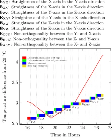
m.Fig. 9illustrates an excerpt from the produced plan for the same 31A. but this time optimising for the uncertainty of measure due to the ordering of the plan. Similarly toFigs. 8 and 9also displays the section of the plan that details the scheduling of interrelated mea-surements. From the plan, it is noticeable that temporal aspects have not been considered because even though measurements using the same instrumentation are grouped together, the planner has scheduled for the instrumentation. It is also noticeable that the plan is optimised to reduce the estimated uncertainty of measure-ment due to the plan order. This can be seen by the fact that the two interrelated straightness errors (EYX and EZY) are scheduled
sequentially followed by the measurement of non-orthogonality between the Y- and X-axis (EC0Y). Scheduling these errors
sequen-tially means that any effect due to changing temperature over time can be minimised. It can also be seen in the produced plan that the temperature variation over the course of the three interrelated measurements is only 0.3°C. The machine downtime when using this error mapping plan would be 34 h and 12 min with a plan order uncertainty of measurement metric of 52
l
m. This plan results in an increased downtime of 1 h over the temporally opti-mised plan, but reduces the uncertainty of measurement metric by 47l
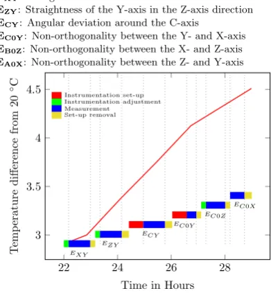
m.The third plan excerpt shown inFig. 10shows the plan order when optimising for both machine tool downtime and the uncer-tainty of measurement due to the plan order for problem instance 31A. Firstly, it is evident that temporal optimisation has been achieved by scheduling measurements that use the same instru-mentation sequentially so that the instruinstru-mentation only needs to
be adjusted, not removed and set-up once again. Secondly, it can be seen that the uncertainty of measurement due to the plan order has been reduced by scheduling interrelated measurements together as well as scheduling them where the temperature differ-ence is at its lowest. From examining the temperature profile seen inFig. 5, it is evident that there are areas where the rate of change of temperature is lower. However, when solving multi-objective optimisation planning problems, a trade-off between both metrics is going to take place. InTable 1this trade-off can be seen where the error mapping plan duration is 33 h 38 min and the uncertainty of measurement metric is 53
l
m. It is evident that both metrics are not as low as when optimising for them individually, but it is clear that the plan is a suitable compromise, showing significant reduc-tion in both machine tool downtime and the uncertainty of mea-surement due to the plan order. In comparison between the single-objective optimum plans, the metrics in the multi-objective plans are on average 2% worse for time and 8% worse for the uncer-tainty of measurement than when they are optimised individually. However, the multi-objective search plans are on average have a 3% reduction in the time metric when compared to the downtime of the uncertainty optimised plan and a 23% improvement in esti-mated uncertainty of measurement metric when compared to the uncertainty of the temporally optimised plan.The graph presented inFig. 11(a) shows the average metrics for the six different three-axis error mapping instances, andFig. 11(b) shows the six different five-axis error mapping instances. In these
Instrumentation set-up Instrumentation adjustment Measurement
Set-up removal
EYX: Straightness of the X-axis in the Y-axis direction EZX: Straightness of the X-axis in the Z-axis direction EZY: Straightness of the Y-axis in the Z-axis direction EXY: Straightness of the Y-axis in the X-axis direction EXZ: Straightness of the Z-axis in the X-axis direction EYZ: Straightness of the Z-axis in the Y-axis direction EC0Y: Non-orthogonality between the Y- and X-axis EB0Z: Non-orthogonality between the Z- and Y-axis EA0Y: Non-orthogonality between the X- and Z-axis
16 18 20 22 24 26 28
2.5
3
3.5
4
EY XEZX EZYEXY
EXZEY Z EC0YEC0Y
EC0Y
Time in Hours
T
emp
erature
d
ifference
from
20
◦C
Fig. 10.Plan excerpt from an uncertainty and temporal optimisation.
[image:9.595.316.559.368.527.2] [image:9.595.317.558.461.712.2]two figures, the effect on both metrics when performing a single-object optimisation can be visualised. Additionally, the trade-off between time and uncertainty when performing the multi-objective optimisation and the compromise in the final solution can easily be visualised. From these two graphs, it can be concluded that performing the multi-objective optimisation is beneficia and adjusted the weighting of each metric would allow optimisation on a case-by-case basis.
7. Conclusions
In this paper it has been identified that in addition to optimising error mapping plans to minimise downtime or the uncertainty of measurement, multi-objective optimisation can be performed. The undertaken case studies show that in comparison between the single-objective optimum plans, the metrics in the multi-objective plans are on average 2% worse for time and 9% worse for the uncertainty of measurement than when they are optimised individually. However, the multi-objective search plans have on average a 3% reduction in the time metric when compared to the downtime of the uncertainty optimised plan and a 23% improve-ment in estimated uncertainty of measureimprove-ment metric when compared to the uncertainty of the temporally optimised plan. Evaluation of the generated plans have validated their fitness-for-purpose and demonstrates the merit of automatically generating measurement plans.
Knowledge regarding the discovery of optimal plans when per-forming the experiments on a PC architecture highlighted that the experimental analysis could be performed on an HPC architecture. These experiments displayed that there is on average a 4% improvement in optimality when compared with the experiments performed on the PC architecture. This warrants the use of the HPC resources for measurement engineers working to sub-micron tol-erances and also suggests that a standard PC architecture is enough for most applications. As the state-of-the-art in both AI autonomous planners and PC computation power improve, the requirement for HPC resources should potentially reduce.
This paper presents novel contributions to both the machine tool metrology and automated planning (AP) community. The first contribution presented in this paper is the ability to use AP to model both temporal and uncertainty of measurement aspects of a machine tool error mapping process. This involved modelling the durations of each individual measurement, as well as discretiz-ing continuous environmental temperature change. The paper then describes how this model can be used by state-of-the-art AP algo-rithms to find optimal plans based on three different metrics. These metrics are: (1) downtime of the machine tool during mea-surement, (2) estimated uncertainty of meamea-surement, and (3) the arithmetic mean of both time and uncertainty. The work under-taken in this paper has also identified that for most manufacturers, using the proposed technology on a standard PC architecture will produce sufficient results. Producing both temporal and estimated uncertainty of measurement optimised plans is a novel contribu-tion to the machine tool metrology community, and provides a solution to the identified literature gap. This has significant impli-cations for all metrological processes where both their cost through downtime, and quality through uncertainty can be reduced. The work presented in this paper is also significant for the AP community as it provides a real-world multi-objective problem to use to initiate the development of more powerful AP tools.
Future work includes the extension of the developed model to account for other continuous factors that affect the uncertainty of measurement. For example, the effect of performing simultaneous measurements on the estimated uncertainty of
measurement needs to be investigated and modelled. This would allow for concurrent measurements to be scheduled to minimise the uncertainty of measurement. Therefore, further reducing machine tool downtime and the uncertainty of measurement.
Acknowledgments
Council (EPSRC) funding of the EPRSC Centre for Innovative Manufacturing in Advance Metrology (Grant Ref: EP/I033424/1). In addition, the authors would like to acknowledge the use of the University of Huddersfield Queensgate Grid in carrying out this work.
References
API. (2014). XD laser – precision laser measurement system. <http:// www.apisensor.com/index.php/products-en/machine-tool-calibration-en/xd-laser-en>, accessed: 2013-06-11.
BIPM. (2008). Evaluation of measurement data – guide to the expression of uncertainty in measurement.
Bohez, E. L. J., Ariyajunya, B., Sinlappcheewa, C., Shein, T. M. M., Lap, D. T., & Belforte, G. (2007). Systematic geometric rigid body error identification of 5-axis milling machines.Computer-Aided Design, 39(4), 229–244.
Bringmann, B., Besuchet, J., & Rohr, L. (2008). Systematic evaluation of calibration methods.CIRP Annals – Manufacturing Technology, 57(1), 529–532.
Bringmann, B., & Knapp, W. (2009). Machine tool calibration: Geometric test uncertainty depends on machine tool performance.Precision Engineering, 33(4), 524–529.
Erol, K., Nau, D. S., & Subrahmanian, V. (1995). Complexity, decidability and undecidability results for domain-independent planning.Artificial Intelligence, 76(1-2), 75–88.
Etalon. (2014). LaserTRACER – measuring sub-micron in space. <http:// www.etalon-ag.com/index.php/en/products/lasertracer>, accessed: 2013-06-03.
Fox, M., Long, D., & Halsey, K. (2004). An investigation into the expressive power of pddl2.1. InECAI(Vol. 16. p. 338).
Fox, M., & Long, D. (2003). PDDL2.1: An extension to PDDL for expressing temporal planning domains.Journal of Artificial Intelligence Research (JAIR), 20, 61–124. Gerevini, A., & Serina, I. (2002). Lpg: A planner based on local search for planning
graphs with action costs. In Proceedings of the artificial intelligence planning systems (AIPS)(Vol. 2. pp. 281–290).
Gerevini, A., Saetti, A., & Serina, I. (2006). An approach to temporal planning and scheduling in domains with predictable exogenous events.Journal of Artificial Intelligence Research (JAIR), 25, 187–231.
Gerevini, A. E., Saetti, A., & Serina, I. (2008). An approach to efficient planning with numerical fluents and multi-criteria plan quality.Artificial Intelligence, 172(8), 899–944.
Ghallab, M., Nau, D., & Traverso, P. (2004).Automated planning: theory & practice. Morgan Kaufmann.
Howey, R., Long, D., & Fox, M. (2004). Val: Automatic plan validation, continuous effects and mixed initiative planning using pddl. In 16th IEEE international conference on tools with artificial intelligence, 2004. ICTAI 2004(pp. 294–301). IEEE.
ISO230. (2005). Part 4: Circular tests for numerically controlled machine tools. ISO230. (2006). Part 2: Determination of accuracy and repeatability of positioning
numerically controlled axes.
ISO230-9. (2005). Estimation of measurement uncertainty for machine tool tests according to series iso 230, basic equations.
Seng Khim, T., & Chin Keong, L. (2010). Modeling the volumetric errors in calibration of five-axis CNC machine. In Proceedings of the international multiconference of engineers and computer scientists (Vol. III, p. 5).
Long, D., & Fox, M. (2003). The 3rd international planning competition: Results and analysis.Journal of Artificial Intelligence Research (JAIR), 20, 1–59.
McDermott, D. M. (2000). The 1998 AI planning systems competition.AI magazine, 21(2), 35.
McDermott, D., Ghallab, M., Howe, A., Knoblock, C., Ram, A., Veloso, M., et al. (1998). PDDL-the planning domain definition language.
Mekid, S. (2009).Introduction to precision machine design and error assessment.No. v. 10 in mechanical engineering series. Taylor & Francis Group.
Mian, N. S., Fletcher, S., Longstaff, A., & Myers, A. (2013). Efficient estimation by {FEA} of machine tool distortion due to environmental temperature perturbations.Precision Engineering, 37(2), 372–379.
Moriwaki, T. (2008). Multi-functional machine tool.CIRP Annals – Manufacturing Technology, 57(2), 736–749.
Muelaner, J. E., Cai, B., & Maropoulos, P. G. (2010). Large-volume metrology instrument selection and measurability analysis.Proceedings of the Institution of Mechanical Engineers, Part B: Journal of Engineering Manufacture, 224(6), 853–868.
twenty-second international conference on automated planning and scheduling. ICAPS 2012 (pp. 216–224). California, USA: AAAI Press.
Parkinson, S., Longstaff, A. P., Crampton, A., & Gregory, P. (2014b). Automated planning for multi-objective machine tool calibration: Optimising makespan and measurement uncertainty. InProceedings of the twenty-fourth international conference on automated planning and scheduling. ICAPS 2012(pp. 421–429). California, USA: AAAI Press.
Parkinson, S., Longstaff, A., & Fletcher, S. (2014a). Automated planning to minimise uncertainty of machine tool calibration.Engineering Applications of Artificial Intelligence.
Parkinson, S., Longstaff, A., Fletcher, S., Crampton, A., & Gregory, P. (2012a). Automatic planning for machine tool calibration: A case study.Expert Systems with Applications, 39(13), 11367–11377.
Russell, S. J., Norvig, P., Canny, J. F., Malik, J. M., & Edwards, D. D. (1995).Artificial intelligence: a modern approach(vol. 74). Prentice hall Englewood Cliffs.
Schwenke, H., Knapp, W., Haitjema, H., Weckenmann, A., Schmitt, R., & Delbressine, F. (2008). Geometric error measurement and compensation of machines - an update.CIRP Annals – Manufacturing Technology, 57(2), 660–675.
Serina, A. G. A. S. I. (2004). Planning with numerical expressions in LPG.Fuel (A1), 100, 50.
Shagluf, A., Longstaff, A., & Fletcher, S. (2013). Towards a downtime cost function to optimise machine tool calibration schedules.Proceedings of the international conference on advanced manufacturing engineering and technologies NEWTECH 2013 (Vol. 16, pp. 231–240). Stockholm, Sweden: KTH Royal Institute of Technology.