A Method for Acquiring the Terminal Common
Mode Impedance of Cables
Hong-yi LIU, Dong-lin SU and Zi-hua ZHAO
School of Electronic and Information Engineering, Beihang University, BeiJing, China
Keywords: Electromagnetic compatibility (EMC), Cable, Terminal impedance, Measurement.
Abstract. A method is presented for quickly acquiring the equivalent terminal common-mode impedance of cables. Firstly, the parallel cables are treated as equivalent multi-conductor transmission line. Using vector network analyzer (VNA) and current probe to measure voltage reflection coefficients at two locations of each cable. Then a nonlinear equation about terminal equivalent impedance is constructed. By solving the nonlinear equations, broadband terminal equivalent impedance for each cable can be acquired. Compared with existing methods, the efficiency of this method is improved significantly. Furthermore, the precision is improved in that this method including the coupling effect between cables. This method helpful to the EMC test and fault diagnosis.
Introduction
The cables connecting the electronic equipment are important coupling path for electromagnetic interference. In order to predict, analyze and solve EMC problems, it is necessary to obtain the common mode input impedance of the cable terminal equipment in a wide frequency band.
In [1]-[3], special circuits are installed into the system to measure impedance. The advantage of these methods is that the accuracy is high. The main shortcoming is that the circuit or instrument will affect the integrity of the system.
In [4]-[7], the current probes are used to measure the impedance of the cable terminals. The advantage of the methods are that the integrity of the system is not affected, and the measurement is simple and convenient. The disadvantage is that the accuracy is affected by the uncertainty of measurement.
For system with cables, the terminal equivalent impedance of each cable is tested one by one by the methods in [1]-[7]. This is not only time consuming, but also does not reflect mutual coupling effect between cables. Therefore, a method is presented for efficiently measuring the common mode equivalent impedance of cable terminal in the paper. Firstly, each multicore cable is equivalent to a single conductor. Then the vector network analyzer and current probe is used to measure the voltage reflection coefficient respectively at two optional locations of each cable. Finally, the equations about equivalent impedances are constructed. The proposed method significantly improves the efficiency of terminal impedance test. On the other hand, the measurement accuracy is improved due to the effects of mutual coupling between the cable is introduced.
Parallel Cables are Equivalent to Multiconductor Transmission Lines
The Equivalent Conductor for a Single Cable
As shown in Figure 2, there are nB conductors in cable B. The conductor i is at the height hi
above ground conductor, radius is Ri. The magnetic conductivity of the media surrounding the conductor is 0, and the dielectric constant is , and the distance between the conductors is far
less than the axial height of the cable. Denote the equivalent conductor above the ground height as
e
h , radius as Re.
ground plane
equipmet1 equipmet2
i h
i
R
e h
e R
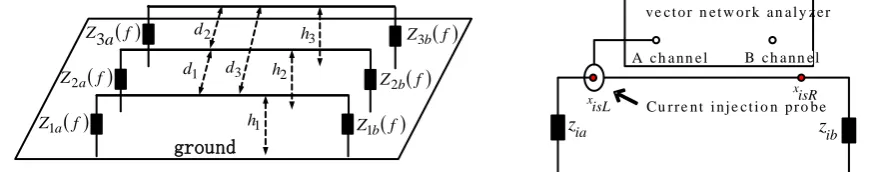
Figure 1. Three wires connecting two terminals. Figure 2. The cross section of a cable and its equivalent conductor.
The inductance of unit length between the conductor i and the ground plane, denoted as lii, is [9]:
2
0 ln
2
hi
lii
Ri
(1)The unit length mutual inductance between conductor A and conductor B is:
0
2
4 ln 1 4
i j ij
ij h h l
d
(2) Assuming that there is current Ii in the conductor i of the cableB, the total magnetic flux B between the unit length cable and the ground plane is:
1
B
n
B ii i
i
l I
(3)Assuming that the magnetic flux between the equivalent conductor and the ground plane is e
when the equivalent conductor carrying 1
B
n i i
I
, the inductance between the equivalent conductor and the ground plane is given:1
B
n
e i e B
i
l I
(4)Substitute (4) into (3), we get:
1 1
1 B
B n
e n ii i
i i i
l l I
I
1
e ii
B i
l l
n
(6)According to (1), for the same le, the he and Re of the equivalent conductor is not unique. For an optional he, Re can be solved by equation (1), get:
2
2 exp
1 0
nB
Re he lii
nB i
(7)
There is the relation of lc 0 for multi conductor transmission line, where l and c is the inductance and the capacitance between the conductor and the ground plane respectively. Therefore, if the equivalent conductors have the same inductance as the cable, they have the same common mode impedance [9].
The Equivalent Conductors for two Parallel Multi-core Cables
On the basis of the equivalent of a single conductor on each cable, the mutual coupling between two parallel cables should be the same as the two equivalent conductors. Set the axes of two parallel multi-core cable B1 and B2 have the height 1
e
B
h and 2
e
B
h above the ground. The cable B1 and
2
B are comprised of conductor Bi1(i1, 2, , 1n ) and B2j(j1,2, , 2n ), respectively. The mutual
inductance between B1i and B2j is denoted as lij. Assuming the conductor i in the cable B1
carrying current Ii, then the magnetic flux 1 2 j B B
between cable B1 and the conductor 2
j
B is:
1 2
1
1
1, 2, , 2
j
n
ij i B B
i
l I j n
(8)The cable B2 can be replaced by an equivalent conductor Be2 on its axis due to the distance
between conductors in cable B2 is very close. Therefore, the equation can be given:
1 2 1 2
2 2 1
1 1 1
2
e j
n n n
ij i
B B B B
j j i
n l I
(9)Now we replace B1 with Be1 and adjust the distance between B1e and Be2 in order to make the mutual inductance 1 2
e e
B B
l to be the equation as follows:
1 2 1 2 1 2
1
1
1
e e e e e
n
i
B B B B B B
i
l I n
(10)Since the distance between the cables is much greater than the distance between the conductors in each of the cables, substitute the formula (10) into equation (9), we get:
1 2
1 2 1 2
1
1 1 1 1
1
1 1
1 2
1 2
e e
n n n n
ij i ij
n B B
i j i j
i i
l l I l
n n
n n I
(11)The distance dij between the two equivalent conductors can be calculated by substituting
1 2
e e
B B
l and 1
e
B
h into (3). For the system shown in Figure 1, by above method, the equivalent
multiconductor transmission line shown in Figure 3 can be achieved. Set the left coordinate of the equivalent conductorxia 0, and the right coordinate xib 2m. According to the method described
conductors d12d210.01m, d130.02m, and the height of the conductor above ground plane
1 2 3 0.025
h h h m. Submitting these values of the equivalent multiconductor transmission line into equation(1), the diagonal elements of the unit length inductance matrix can be achieved. Similarly, submitting these values into equation(3), the non-diagonal element of the unit length inductance matrix can be achieved. Therefore, the characteristic impedance matrix Zc L 0 0 can be
achieved. In Figure 3, zia
f and zib
f are the equivalent impedance of the left and right end of the cables, respectively.Acquiring the Input Impedance Matrix of the Multiconductor Transmission Line
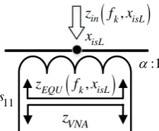
To obtain zia
f and zib
f , the input impedance array of the transmission line at two optional positions is required. The measurement method is shows in Figure 4. The current probe is connected to the A channel of the vector network analyzer, and the current probe is installed at the optional position x1sL near the left terminal of the conductor 1. Then, the vector network analyzer sweeps frequency at the m frequencies, and the m voltage reflection coefficients is obtained, which is written as
1
1
,
L k sL m
s f x
, where sL
fk,x1sL
is the voltage reflection coefficient at the frequency fk. The current probe is installed at x1sR near the right terminal of conductor 1, and then sweeps frequency once again. Then another set of voltage reflection coefficients are obtained, which is recorded as
1
1
,
R k sR m
s f x
, where sR
fk,x1sR
is the voltage reflection coefficient at frequency fk. For conductors 2 and 3, repeat above process, the voltage reflection coefficient matrix
,
3L k isL m
s f x
and
3
,
R k isR m
s f x
can be obtained. To calculate the input impedances at
isL
x and xisR of the equivalent conductor, the equivalent circuit of the current probe and the measured conductor should be established. The equivalent circuit of the current probe and the conductor in Figure 4 is shown in Figure 5.
ground 1
h
2
h
3 h 2
d
3 d
f Z1a
f Z2a
f a Z3
f Z1b
f Z2b
f Z3b
1
d
A c h a n n e l B c h a n n e l v e c t o r n e t w o r k a n a l y z e r
Cu r r e n t i n j e c t i o n p r o b e
ia z
ib z
[image:4.595.50.495.449.535.2]xisL xisR
Figure 3. The equivalent MTL of the three cables. Figure 4. Testing voltage reflection coefficient of the conductor i.
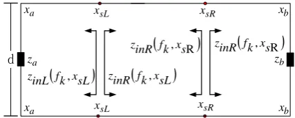
In Figure 5, zVNA 50 is the input impedance of the vector network analyzer channel A, and
,
in k isL
z f x is the input impedance of the conductor at xisL and on the frequency fk. According to the circuit theory, the equivalent impedance at the connection of the current probe and the vector
network analyzer is zEQU
fk,xisL
2zin
fk,xisL
, and the voltage reflection coefficient
,
L k isL
s f x is[9] :
2 2
, ,
, +
in k isL VNA
L k isL
in k isL VNA
z f x z
s f x
z f x z
(12)
,
in k isL z f xisL x
:1
, isL
EQU kz f x
VNA
z 11
[image:5.595.241.354.71.164.2]s
Figure 5. The equivalent circuit for measuring the voltage reflection coefficient of a conductor.
According to (12), we get:
L 2
L
1 ,
,
1 ,
VNA L k is
in k isL
L k is
z s f x
z f x
s f x
(13) Similarly, the input impedance of conductor i at xisR is presented as follow:
2
1 ,
,
1 ,
VNA R k isR
in k isR
R k isR
z s f x
z f x
s f x
(14) For the three conductors, repeatedly use (13) and (14) at mfrequencies. Then the input
impedance matrixes at XsL
x1sL,x2sL,x3sL
and XsR
x1sR,x2sR,x3sR
can be obtained:
,
,
3
Zin f XsL zin fk xisL
m
(15)
,
,
3
Zin f XsR zin fk xisR
m
(16) In (15) and (16),
z
in
f
k,
x
isL
and zin
fk,xisR
is the element of line i and column k, respectively.Calculating the Terminal Impedance
As shown in Figure 6, if the frequency of the injected signal with current probe is fk, we denote
,
inL k sL
z f x as the input impedance when looking from xsL towards left, and zinR
fk,xsL
isthe input impedance when looking from xsL towards right. Similarly, zinL
fk,xsR
is the inputimpedance when looking from xsR towards left, and
z
inR
f
k,
x
sR
is the input impedance when looking from xsR towards right. The mutual coupling between conductors can be ignored if the conductor spacing of the equivalent multiconductor is large. Therefore the formulas are given:
1,
inL k sL c a k c k sL a c a k k sL a
z f x z z f jz tg x x z jz f tg x x (17)
1,
inR k sL c b k c k b sL c b k k b sL
z f x z z f jz tg x x z jz f tg x x (18)
1R R R
,
inL k s c a k c k s a c a k k s a
z f x z z f jz tg x x z jz f tg x x (19)
1R R R
,
inR k s c b k c k b s c b k k b s
a
x xsL xb
a
z zb
sR
x
fk xsL
inL z ,
fk,xsR
inR z
fk xsL
inR z ,
fk,xsR
inR z d
sL
x xsR
a
[image:6.595.191.405.70.156.2]x xb
Figure 6. Four input impedances between conductor and ground.
In (17)-(20), k 2fk c, where c is the speed of light, zc is the characteristic impedance between the conductor i and ground plane, which can be calculated by the inductance obtained from (1) multiplying 1 0 0[9]. There are mutual coupling effects if the conductors of the equivalent multiconductor transmission line are close. Therefore (17)-(20) should be improved as the equations:
, X
inL k sL c a k c k sL a c a k k sL a
Z f Z Z f jZ tg X X Z jZ f tg X X (21)
, X
inR k sL c b k c k b sL c b k k b sL
Z f Z Z f jZ tg X X Z jZ f tg X X (22)
, X
inL k sR c a k c k sR a c a k k sR a
Z f Z Z f jZ tg X X Z jZ f tg X X (23)
, X
inR k sR c b k c k b sR c b k k b sR
Z f Z Z f jZ tg X X Z jZ f tg X X (24) In (21) -(24), Za
fk and Zb
fk is diagonal matrix. Their diagonal elements are the unknownvariable zia
fk and zib
fk
i1, 2,3
, respectively. Xa
xia 3 1 and Xb
xib 3 1 is column vector constructed by the coordinates of the left and right terminal. tgk
XsL -Xa
,
-
k b sL
tg X X , tgk
XsR -Xa
and tgk
Xb -XsR
is the tangent matrix of phase difference between the observation point and the terminal, which are given by:
1 1 2 1 3 1
1 2 2 2 3 2
1 3 2 3 3 3
k sL a k sL a k sL a
k sL a k sL a k sL a k sL a
k sL a k sL a k sL a
tg x x tg x x tg x x
tg X X tg x x tg x x tg x x
tg x x g x x tg x x
(25)
1 1 1 2 1 3
2 1 2 2 2 3
3 1 3 2 3 3
k b sL k b sL k b sL
k b sL k b sL k b sL k b sL
k b sL k b sL k b sL
tg x x tg x x tg x x
tg X X tg x x tg x x tg x x
tg x x g x x tg x x
(26)
1 1 2 1 3 1
1 2 2 2 3 2
1 3 2 3 3 3
k sR a k sR a k sR a
k sR a k sR a k sR a k sR a
k sR a k sR a k sR a
tg x x tg x x tg x x
tg X X tg x x tg x x tg x x
tg x x tg x x tg x x
(27)
1 1 1 2 1 3
2 1 2 2 2 3
3 1 3 2 3 3
k b sR k b sR k b sR
k b sR k b sR k b sR k b sR
k b sR k b sR k b sR
tg x x tg x x tg x x
tg X X tg x x tg x x tg x x
tg x x g x x tg x x
(28)
The input impedance matrix Zin
f X, sL
at XsL and the input impedance matrix
,
in sR
Z f X at XsR can be calculated by:
-1
, , , , ,
in sL inL k sL inR k sL inL k sL inR k sL
k
in k, sR
inL
k, sR
inR
k, sR
inL
k, sR
inR
k, sR
k
col um Z f X diag Z f X Z f X Z f X Z f X (30) In (29) and (30),
k
colum is the kth column vector of a matrix, diag
is the column vectorconstructed by the diagonal elements of a matrix. For each value of k, (29) and (30) constitute equations about the six unknown terminal impedances. The equations can be solved by the trust region dogleg algorithm as below:
Step 0: Set k1.
Step 1: Set z1a,z2a,z3a,z1b,z2b and z3b initial values that are greater than zero. According to
(29) and (30), a six dimensional column vector equation 1
2
=0
F F
F
is constructed, where F1 and
2
F is defined by:
1
1 in , sL inL k, sL inR k, sL inL k, sL inR k, sL
k
F colum Z f X diag Z f X Z f X Z f X Z f X (31)
1
2 in k, sR inL k, sR inR k, sR inL k, sR inR k, sR
k
F colum Z f X diag Z f X Z f X Z f X Z f X (32)
Step 2: Substituting z1a,z2a,z3a,z1b,z2band z3b into(31)and(32), the six dimensional column vector F can be obtained.
Step 3: Calculate the 2-norm F 2, then judge F 2 to be true or false. The is a predetermined small positive number as the condition of terminating iteration. In this paper,
-8
10
. If F 2 , then z1a ,z2a,z3a,z1b ,z2b and z3b is the terminal impedance at fk . Otherwise execute step 4.
Step 4: Execute iteration one step on the vector equation F by the trust region dogleg algorithm, the new values of z1a,z2a,z3a,z1b,z2bandz3b are obtained. Then return to Step 2.
Step 5: Set k k 1. If km, return to step. Otherwise, end loops.
The Experimental Results
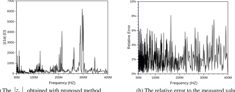
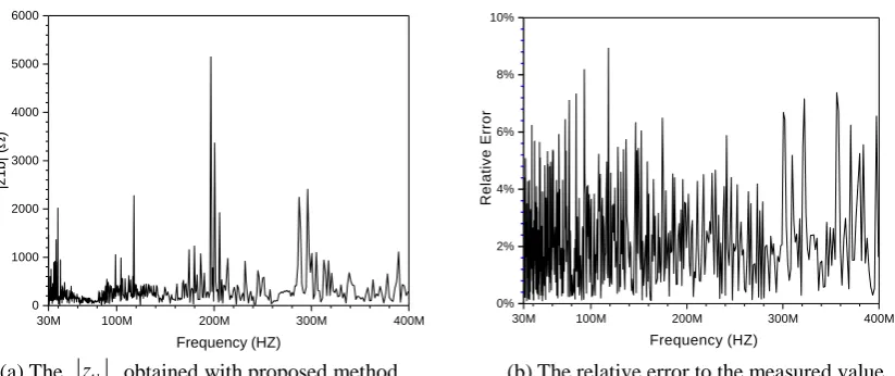
Without loss of generality, set xisL0.2m, xisR1.7m. According to CS114, 520 frequencies were selected 30MHz-400MHz. According to part 2, six groups of voltage reflection coefficients were acquired. According to part 3, two terminal impedance matrix of 3 line by 520 columns were obtained. In figure 7(a)-12 (a), six terminal impedances obtained by the proposed method in this paper are shown. In figure 7(b)-12 (b), the relative errors between the value obtained by the proposed method and measured by an impedance analyzer are given. As shown in these figures, the relative error is less than 5%, which is far below the uncertainty of the measurement.
100M 200M 300M
30M 400M
0 1000 2000 3000 4000 5000 6000 7000
|z
1
a
|
(
)
Frequency (HZ)
100M 200M 300M
30M 400M
0% 2% 4% 6% 8% 10%
R
e
lati
v
e
E
rr
o
r
Frequency (HZ)
(a) The z1a obtained with proposed method (b) The relative error to the measured value
[image:7.595.99.500.603.761.2]100M 200M 300M
30M 400M
0 1000 2000 3000 4000 5000 6000 7000 8000 9000 10000 11000 12000
|z
2
a
|
(
)
Frequency (HZ)
100M 200M 300M
30M 400M
0% 2% 4% 6% 8% 10%
R
e
lati
v
e
E
rr
o
r
Frequency (HZ)
[image:8.595.107.492.69.224.2](a) The z2a obtained with proposed method (b) The relative error to the measured value
Figure 8. The z2a achieved with proposed method and its relative error to measured value.
100M 200M 300M
30M 400M
0 1000 2000 3000 4000 5000 6000 7000 8000 9000 10000
|z
3
a
|
(
)
Frequency (HZ)
100M 200M 300M
30M 400M
0% 1% 2% 3% 4% 5% 6% 7% 8% 9% 10%
R
e
lati
v
e
E
rr
o
r
Frequency (HZ)
[image:8.595.95.500.255.429.2](a) The z3a obtained with proposed method (b) The relative error to the measured value
Figure 9. The z3a achieved with proposed method and its relative error to measured value.
100M 200M 300M
30M 400M
0 1000 2000 3000 4000 5000 6000
|z
1
b
|
(
)
Frequency (HZ)
100M 200M 300M
30M 400M
0% 2% 4% 6% 8% 10%
R
e
lati
v
e
E
rr
o
r
Frequency (HZ)
(a) The z1b obtained with proposed method (b) The relative error to the measured value
[image:8.595.94.506.460.633.2]100M 200M 300M
30M 400M
0 1000 2000 3000 4000 5000 6000 7000 8000 9000 10000 11000
|z
2
b
|
(
)
Frequency (HZ)
100M 200M 300M
30M 400M
0% 2% 4% 6% 8% 10%
R
e
lati
v
e
E
rr
o
r
Frequency (HZ)
[image:9.595.94.513.71.247.2](a) The z2b obtained with proposed method (b) The relative error to the measured value
Figure 11. The z2b achieved with proposed method and thus its relative error to measured value.
100M 200M 300M
30M 400M
0 1000 2000 3000
|z
3
b
|
(
)
Frequency (HZ)
100M 200M 300M
0M 400M
0% 1% 2% 3% 4% 5% 6% 7% 8% 9% 10%
R
e
lati
v
e
E
rr
o
r
Frequency (HZ)
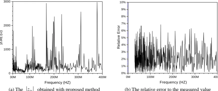
(a) The z3b obtained with proposed method (b) The relative error to the measured value
Figure 12. The z3b achieved with proposed method and thus its relative error to measured value.
Conclusion
According to the method proposed in this paper, the equivalent common mode impedance of the cable terminals can be tested quickly. The relative error between the values obtained by the proposed method and by direct measurement with impedance analyzer are less than 10% at most of frequencies. Therefore, this method can meet the precision needed by electromagnetic compatibility engineering. By the method in this paper, the equivalent common mode impedance can be obtained efficiently, which is helpful for the system level EMC testing and troubleshooting.
References
[1] Huang W, Qahouq J A A. An Online Battery Impedance Measurement Method Using DC–DC Power Converter Control[J]. IEEE Transactions on Industrial Electronics, 2014, 61(11):5987-5995.
[2] Yang Zhen, Zhang Jianfeng. Research on sinusoidal impedance measurement method of square wave current injection based on [J]. Shaanxi Electric Power, 2014, 42 (12): 39-43.(in Chinese)
[3] Yue dragons, Zhuo Fang, Zhang Zhenghua, et al. Measurement of electronic power system impedance section two fork tree [J]. Journal of Electric Technology, 2015, 30 (24): 76-83. (in Chinese)
[image:9.595.76.516.282.467.2][J]. Measurement and Control Technology,2014,33 (supplement): 364-370. (in Chinese)
[5] Zhao Hongxu, Wang Qian, Wang Jialin. Design and implementation of loop impedance measurement system for aircraft cable shield [J]. Automation Instrument, 2016, 37 (12): 40-44. (in Chinese)
[6] See K Y, Deng J. Measurement of noise source impedance of SMPS using a two probes approach[J]. IEEE Transactions on Power Electronics, 2004, 19(3):862-868.
[7] Tan J, Zhao D, Ferreira B. A method for in-situ measurement of grid impedance and load impedance at 2 k–150 kHz[C]//Power Electronics and ECCE Asia (ICPE-ECCE Asia), 2015 9th International Conference on. Seoul: IEEE, 2015: 443-448.
[8] Powell M J D. A FORTRAN subroutine for solving systems of nonlinear algebraic equations. No. AERE-R--5947 [R]. Harwell (England): Atomic Energy Research Establishment, 1968.
[9] Paul. Multi-conductor transmission line analysis, [M]. (Second Edition). Beijing: China Electric Power Press, 2013:62-283(in Chinese)