Global Imbalances: Should We Use Fundamental Equilibrium Exchange Rates?

Munich Personal RePEc Archive

Global Imbalances: Should We Use

Fundamental Equilibrium Exchange

Rates?

Saadaoui, Jamel

University of Paris North

10 November 2012

Online at

https://mpra.ub.uni-muenchen.de/42554/

Global Imbalances: Should We Use Fundamental

Equilibrium Exchange Rates?

∗

Jamel Saadaoui

November 10, 2012

Abstract

The reduction of global imbalances observed during the climax of crisis is incom-plete. In this context, currencies realignments are still proposed to ensure global macroeconomic stability. These realignments are based on equilibrium rates de-rived from equilibrium exchange rate models. Among these models, we have the fundamental equilibrium exchange rate (FEER) model introduced byWilliamson

(1994). This approach is often labelled as normative mainly because the return to the equilibrium is not described in the model. If the FEER is not related neither in the short nor in the long to the real exchange rates, we see no clear justification to intervene in foreign exchange markets based on these equilibrium rates. In this case, the FEER is a normative approach and should not be used to reduce global imbalances. This paper provides empirical evidences robust to cross-sectional de-pendence that the FEER is related to real exchange rate in the long run and thus could be a useful tool to prevent the resurgence of large global imbalances and associated risks.

JEL Classification:F31, F41.

Key words: Global Imbalances, Equilibrium Exchange Rate, International Monetary Cooperation.

∗_{The author is grateful to Gian Maria Milesi-Ferretti for providing updated data of net foreign assets.} †_{PhD candidate, Center of Economics of Paris North, CNRS Mixed Research Unit n}o_{7234, University}

1

Introduction

As witnessed by the evolution of current account balances and net foreign assets, the re-duction of global imbalances observed during the climax of crisis is incomplete. Indeed, current account imbalances in flow have been reduced with the global slowdown and the collapse of the world trade in 2009. However, these evolutions of current account im-balances have not been sufficient to reduce net foreign assets positions in stock. After the climax of the crisis, global imbalances in stock (i.e. the net foreign assets positions) represent more than 15% of world GDP in absolute value as we can see in Fig. 1.

Fig. 1: Net foreign assets (in percent of world GDP)

-25 -20 -15 -10 -5 0 5 10 15 20

2000 2001 2002 2003 2004 2005 2006 2007 2008 2009 2010 2011

US JPN Eur surplus CHN EMA

OIL ROW Eur deficit Discrepancy

Note: Data are preliminary for 2011. EUR surplus: Austria, Belgium, Denmark, Finland, Germany, Luxembourg, Netherlands, Sweden, Switzerland. EUR deficit: Greece, Ireland, Italy, Portugal, Spain,

United Kingdom, Bulgaria, Czech Republic, Estonia, Hungary, Latvia, Lithuania, Poland, Romania, Slovak Republic, Turkey, Ukraine. Emerging Asia: Hong Kong S.A.R. of China, Indonesia, Korea, Malaysia, Philippines, Singapore, Taiwan province of China, Thailand. Oil exporters: Algeria, Angola, Azerbaijan, Bahrain, Republic of Congo, Ecuador, Equatorial Guinea, Gabon, Iran, Kazakhstan, Kuwait, Libya, Nigeria, Norway, Oman, Qatar, Russia, Saudi Arabia, Sudan, Syria, Trinidad and Tobago, United

Arab Emirates, Venezuela, Yemen. Rest of the world: remaining countries.

economy. Firstly, large current account imbalances increase the systemic risks as coun-tries with large deficits can be subject to sudden stops and their macroeconomic conse-quences. Secondly, they increase political tensions as a number of countries, which are suspected of unfair competition with undervalued exchange rates, could be threatened by retaliatory measures. Thirdly, in the current context of weak growth in advanced countries, the perpetuation of export-led growth strategies in some emerging countries could be a menace for the global recovery.

Currencies realignments are still proposed to ensure global macroeconomic stability. These realignments are based on equilibrium rates derived from equilibrium exchange rate models. Among these models, we have the fundamental equilibrium exchange rate (FEER) model introduced by Williamson (1994). This approach is often labelled as normative mainly because the return to the equilibrium is not described in the model. If the FEER is not related neither in the short nor in the long to the real exchange rates, we see no clear justification to intervene in foreign exchange markets based on these equilibrium rates. In this case, the FEER is a normative approach and should not be used to reduce global imbalances. This paper provides empirical evidences robust to cross-sectional dependence that the FEER is related to real exchange rate in the long run and thus could be a useful tool to prevent the resurgence of large global imbalances and associated risks.

This paper is organized as follow. Section 2 presents a general framework of the FEER approach. Sections 3 focusses on the empirical results robust to cross-sectional depen-dence. Section 4 concludes on the usefulness of the FEER approach to reduce global imbalances.

2

FEER Methodology

In the literature on equilibrium exchange rates, the FEER approach have several vari-ants. We can quoteCline(2008), Jeong et al.(2010) andCarton and Herv´e(2012) for example. These variants differs on the type and size of modelling (general equilibrium, partial equilibrium, reduced form relationship), on the determination of the sustainable current account in the medium term (econometric estimates, judgemental assessment, arithmetic average) and on the trade elasticities (calibration to balance the trade model in volume and value, econometric estimates in a panel setting to ensure consistency of the world trade model).

In spite of all these differences, we present a general framework adapted to describe every FEER approach. We start with a simple current account model based on Clark and MacDonald(1998):

CA=−KA (1)

ntb=b0+b1q+b2yd pot+b3y f pot (3)

n f ar= f(q) (4) WhereCAis the current account balance,KAis the capital account,ntbis the net trade balance, n f ar represents returns of net foreign assets, q is the real effective exchange rate (when qincreases, we observe a real effective depreciation), yd pot is the domes-tic full employment output and y f pot represents full employments output of foreign economies.

A real effective depreciation and an increase of full employments output of foreign economies improve the net trade balance (b1>0,b3>0), an increase of the domestic

full employment output deteriorates the net trade balance (b2<0).

Combining Equations1to4gives:

CA∗= f(qreer,yd pot,y f pot) =−KA∗ (5)

WhereCA∗is the sustainable current account in the medium term.

To determine the FEER, every approach have to solve the following equation:

qf eer= f(KA∗,yd pot,y f pot) (6)

We obtain the fundamental equilibrium exchange rate (qf eer), which realizes simultane-ously the external and internal equilibrium for all trading partners.

In our approach, we use a two-step procedure to obtain the fundamental equilibrium exchange rate for each trading partners (Jeong et al., 2010). Firstly, we use a partial equilibrium model of world trade for the main countries at the world level (US, China, Japan, Euro area, UK and the Rest of the World). We solve Equation6 to obtain fun-damental equilibrium exchange rates for these countries in a partial equilibrium model of 35 equations. Secondly, we use simple national model in which world demand and world price are exogenous for smaller economies. National estimates are linked with the estimates of the main countries at the world level1. In that case the misalignments (i.e. the difference between observed rates and equilibrium rates), written in differential logarithmic (r=dLogR= (Ri−Re)/Re_{), are computed as}2_:

r= 1

sx.

b

mx+ηm.di−ηx.d

∗ ₍₇₎

Wherebis the difference between the observed current account and the equilibrium one, as percentage of GDP, d andd∗ stand for internal and world demand in volume, also

1_{Notice that the FEER estimates are not obtained country-by-country but in a consistent framework}

by relying on a world trade model for the main economic areas.

written in differential logarithmic, ηm and ηx are import and export volume elastici-ties,sxandmxare coefficients derived from the foreign trade model in which mark-up behaviours are allowed.

Concerning the determination of the sustainable current account in the medium term, following (Chinn and Prasad,2003), we regress the current account on several medium-term demedium-terminants of investment and saving behaviours. The consistency of current account targets is ensured by using the Rest of the World as a residual. At the world level, the sum of current account targets expressed in the same currency is equal to zero. The trade elasticities of the world trade model comes from econometric estimates. These estimates are generally made in a panel setting to ensure that elasticities are mutually consistent3.

Although, there are several variants of the FEER approach in the literature on equilib-rium exchange rates. This simplified framework contains the essential principles which are included in all FEER approaches.

3

Empirical Results

The purpose of this section is twofold. First, we estimate FEERs for seventeen in-dustrialized and emerging countries (the United States, the United-Kingdom, the Euro area, Japan, Korea, China, Brazil, India, Mexico, Argentina, Chile, Colombia, Indone-sia, MalayIndone-sia, Philippines, Thailand and Uruguay) over the period 1982 to 2007 with the methodology described above4. Secondly, we test empirically the usefulness of the FEER approach to reduce global imbalances.

After the estimation of FEERs for these seventeen countries over the period 1982-2007, we test the following long-run relationships:

reeri,t=αi+βf eeri,t+µi,t (8)

f eeri,t =δi+θreeri,t+εi,t (9)

Where f eeris the fundamental equilibrium exchange rate andreeris the real effective exchange rate5. Variables in minuscule represents natural logarithms.

When the time dimension (T =26 in our sample) is superior to the cross-section dimen-sion (N=17 in our sample), we can test the existence of cross-sectional dependencies with a Lagrange multiplier test as pointed out byDe Hoyos and Sarafidis(2006). Con-sequently, we apply an LM test on an ARDL(1,1) specification with fixed effects as in

Persyn and Westerlund(2008).

3_{SeeJeong et al.(2010) for more details and complete description of the model and the methodology.} 4_{Estimates for emerging countries are presented and discussed inAflouk et al.(2010).}

Table 1: Breusch-Pagan LM test of independence

p-value Equation (8) 0.000 Equation (9) 0.000

Source: author’s calculations.

As we can see in Table1, we strongly reject the null hypothesis of cross-sectional inde-pendence. In order to take into account cross-sectional dependence, we implement panel unit root tests, panel cointegration tests and a new estimator which allow cross-sectional dependence.

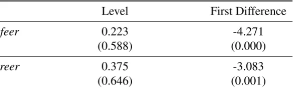
We use the CADF test introduced byPesaran(2007) to test the unit root properties of the variables in presence of cross-sectional dependence. This test is robust to cross section dependencies by subtracting cross section averages of lagged levels in addition to the standard ADF equation. As shown by Table2, series are nonstationary I(1) series as a I(1) series achieves stationarity after first differencing.

Table 2: Integration of the variables

Level First Difference

feer 0.223 -4.271

(0.588) (0.000)

reer 0.375 -3.083

(0.646) (0.001)

Source: author’s calculations. Note:p-values in parentheses.

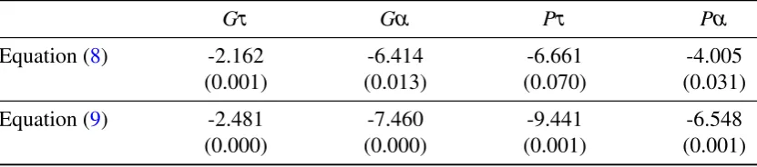
To test cointegration, we use the panel and the ”mean group” statistics suggested by

Table 3: Cointegration of the variables

Gτ Gα Pτ Pα

Equation (8) -2.162 -6.414 -6.661 -4.005 (0.001) (0.013) (0.070) (0.031)

Equation (9) -2.481 -7.460 -9.441 -6.548 (0.000) (0.000) (0.001) (0.001)

Source: author’s calculations. Notes: p-values in parentheses. p-values for cointegration tests are based on bootstrap methods, where 800 replications are used. SeePersyn and Westerlund(2008) for the details.

et al., 1999) with cross sectional average of independent and dependent variables in order to capture the common factors or the heterogeneous time effects.

More precisely, we start with the ARDL(1, 1) model as specified in Equation10:

reeri,t =δ0i+δ1if eeri,t+δ2if eeri,t−1+λireeri,t−1+ui,t (10)

The error correction equation yield:

∆reeri,t=φi(reeri,t−1−θ0i−θ1if eeri,t)−δ2i∆f eeri,t+ui,t (11)

Now, we assume that the error termui,t follow multi-factor error structure:

ui,t=γift+εi,t (12)

where ftis a factor of unobserved common shocks. The error terms dependencies across

individuals are captured by f, whereas the impacts of these factors on each country are governed by the idiosyncratic loadings inγi.

By using Equations10and12and by averaging across i, we obtain:

reert=δ¯0+δ¯1f eert+δ¯2f eert−1+λ¯reert−1+γ¯ft+ε¯t (13)

Where the variables with a bar denote the simple cross section averages of the corre-sponding variables in year t. The common factors can be captured through a linear combination of the cross-sectional averages of the dependent variable and of the regres-sors:

γift=−ciδ¯0−ci δ¯1+δ¯2

whereci=γ_γ¯i. Replacing Equations12and14in Equation11yields the error correction

equation:

∆reeri,t=φi reeri,t−1−θ0i−θ1if eeri,t−a∗ireert−1+b∗i f eert

−δ2i∆f eeri,t+ci∆reert+c∗i∆f eert+εi,t (15)

Where φi = −(1−λi); θ0i = δ0i−ciδ¯0/(1−λi); θ1i = (δ1i+δ2i)/(1−λi); a∗_i = ci 1−λ¯

/(1−λi);b∗_i =ci δ¯1+δ¯2

/(1−λi);c∗_i =ciδ¯2.

Since the CPMG estimator imposes long-run coefficients to be constant for all individ-uals, while it allows short run heterogeneity, the error correction models6are written:

∆reeri,t=φ reeri,t−1−θ0−θ1f eeri,t−a∗reert−1+b∗f eert

−δ2i∆f eeri,t+ci∆reert+c∗i∆f eert+εi,t (16)

∆f eeri,t =φ f eeri,t−1−θ0−θ1reeri,t−a∗f eert−1+b∗reert

−δ2i∆reeri,t+ci∆f eert+c∗i∆reert+εi,t (17)

The results are presented in Tables4and6. The estimations give clear cut results. They clearly show a positive and significant long-run relationship between fundamental rates and observed rates in presence of cross-sectional dependence. The results are robust to different groups of countries since the results in Tables5and7are very similar to those for the entire sample.

As pointed out by Saadaoui (2011), in case of cyclical evolution of competitiveness (Equation8), the half-life7is equal to 3.8 years (3 years for emerging countries only). For structural evolution of competitiveness (Equation 9), the half-life is equal to 2.31 years (2.15 years for emerging countries only). When a country experienced a cycli-cal evolution of its competitiveness, it can slow the return to equilibrium in case of unfavourable evolutions hence a longer half-life8.

We provide robust empirical evidences that the FEER approach is related in the long run with observed rates even if the dynamic of real exchange rates is not explicitly described in the model. These results confirm the usefulness of the FEER approach to reduce global imbalances. The FEER approach should be used as a tool to prevent the return of large imbalances and associated risks.

6_{Causality tests have been conducted thanks to the Pooled Mean Group estimator. They clearly show}

that the causal relationship is bi-directional (Saadaoui,2011).

7 _{The half-lives are computed by using the following formula: h=−ln(0.5)/ln(1+|φ|). They}

correspond to the number of periods for a deviation (from the long run equilibrium) to decay by 50%. Here, deviations correspond to misalignments.

Table 4: Long-relationship (Equation8)

Long-run coefficient (β) z-stat / p-value

CPMG 0.53*** 7.38

Error-correction term (φ) -0.20*** -4.27

Hausman test 1.13 0.77

Number of cross-section 17

Number of periods 26

Number of observations 442

Source: author’s calculations. Notes: p-value for the Hausman test of homogeneity of long run coefficients. The symbol *** indicates statistical significance at the 1% level.

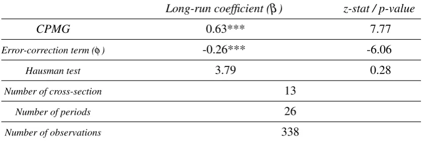
Table 5: Long-relationship (Equation8) for emerging countries only

Long-run coefficient (β) z-stat / p-value

CPMG 0.63*** 7.77

Error-correction term (φ) -0.26*** -6.06

Hausman test 3.79 0.28

Number of cross-section 13

Number of periods 26

Number of observations 338

Table 6: Long-relationship (Equation9)

Long-run coefficient (θ) z-stat / p-value

CPMG 0.64*** 13.37

Error-correction term (φ) -0.35*** -6.72

Hausman test 1.57 0.66

Number of cross-section 17

Number of periods 26

Number of observations 442

Source: author’s calculations. Notes: p-value for the Hausman test of homogeneity of long run coefficients. The symbol *** indicates statistical significance at the 1% level.

Table 7: Long-relationship (Equation9) for emerging countries only

Long-run coefficient (θ) z-stat / p-value

CPMG 0.73*** 11.29

Error-correction term (φ) -0.38*** -5.21

Hausman test 2.57 0.46

Number of cross-section 13

Number of periods 26

Number of observations 338

4

Conclusion

The reduction of global imbalances observed during the climax of crisis is incomplete as witnessed by the evolution of net foreign assets positions. In this context, currencies realignments are still proposed to ensure global macroeconomic stability. These curren-cies realignments are based on equilibrium (or reference) rates derived from equilibrium exchange rate models. Among these models, we have the FEER approach introduced by Williamson (1994). This approach is often labelled as normative as the exchange rate dynamic is not explicitly described in the model. We provide robust empirical evi-dences that fundamental rates are related in the long run with observed rates in presence of cross-section dependence. These empirical results are supportive of the usefulness of the FEER approach to reduce global imbalances and associated risks. A return of large imbalances could dampen the global recovery (Blanchard and Milesi-Ferretti,2012). In July 12, the IMF has adopted the FEER concept to strengthen its surveillance ac-tivities on bilateral and multilateral levels (International Monetary Fund, 2012). In its

Pilot External Sector Report, the IMF produce a set of deviations between real effec-tive exchange rates and those consistent with fundamental and desirable policies for 28 economies. Even if this new decision does not create new formal obligations, it could be considered as a step in the recognition that members must have mutually consistent objectives to ensure global macroeconomic and macrofinancial stability.

References

Aflouk, N., S.-E. Jeong, J. Mazier, and J. Saadaoui (2010). Exchange rate misalignments and international imbalances: a FEER approach for emerging countries. Economie´ Internationale 124, 31–74.

Blanchard, O. and G. M. Milesi-Ferretti (2012). (Why) Should current account balances be reduced? IMF Economic Review 60, 139–150.

Carton, B. and K. Herv´e (2012). Estimation of consistent multi-country FEERs. Eco-nomic Modelling 29, 1205–1214.

Chinn, M. D. and E. Prasad (2003). Medium term determinants of current accounts in industrial and developing countries: an empirical exploration. Journal of Interna-tional Economics 59, 47–76.

Clark, P. and R. MacDonald (1998). Exchange rates and economic fundamentals - a methodological comparison of BEERs and FEERs. Working paper 98/67, Interna-tional Monetary Fund.

Cline, W. R. (2008). Estimating consistent fundamental equilibrium exchange rates. Working paper 08-6, Peterson Institute for International Economics.

De Hoyos, R. E. and V. Sarafidis (2006). Testing for cross-sectional dependence in panel-data models. Stata Journal 6, 482–496.

International Monetary Fund (2012). Pilot external sector report. Technical report, International Monetary Fund.

Jeong, S.-E., J. Mazier, and J. Saadaoui (2010). Exchange rate misalignments at world and European levels: a FEER approach. Economie Internationale 121´ , 25–58.

Mohaddes, K., M. Raissi, and T. Cavalcanti (2012). Commodity price volatility and the sources of growth. Working paper 12/12, International Monetary Fund.

Persyn, D. and J. Westerlund (2008). Error-correction based cointegration tests for panel data. Stata Journal 8, 232–241.

Pesaran, M. H. (2006). Estimation and inference in large heterogeneous panels with a multifactor error structure. Econometrica 74, 967–1012.

Pesaran, M. H., Y. Shin, and R. P. Smith (1999). Pooled mean group estimation of dynamic heterogeneous panels. Journal of the American Statistical Association 94, 621–634.

Saadaoui, J. (2011). Exchange rate dynamics and fundamental equilibrium exchange rates. Economics Bulletin 31, 1993–2005.

Westerlund, J. (2007). Testing for error correction in panel data. Oxford Bulletin of Economics and Statistics 69, 709–748.