Effect of Partially Coherent Light on the Contrast of Speckle Patterns Obtained Using Digital Image Processing of Speckle Photography

(1)

Effect of Partially Coherent Light on the Contrast of

Speckle Patterns Obtained Using Digital Image

Processing of Speckle Photography

Nasser A. Moustafa, Mohamad M. El-Nicklawy, Amin F. Hassan, Amany K. Ibrahim Department of Physics, Faculty of Science, Helwan University, Cairo, Egypt

Email: [email protected]

Received May 13, 2013; revised June 17, 2013; accepted July 12, 2013

Copyright © 2013 Nasser A. Moustafa et al. This is an open access article distributed under the Creative Commons Attribution Li-cense, which permits unrestricted use, distribution, and reproduction in any medium, provided the original work is properly cited.

ABSTRACT

The paper is devoted to study theoretically, the effects of some parameters on the visibility of the speckle patterns. For this propose, a theoretical model for a periodic rough surface was considered. Using this theoretical model, the effects of grain height, its density, the band width and spectral distribution of the line profile (Gaussian and Lorentzian) illu-minating a rough surface on the visibility of speckle pattern are investigated. An experimental setup was constructed to study the effect of surface roughness and coherence of the illuminating light beam on the contrast of speckle pattern. The general behavior of the experimental results, which agree with published data, is compatible with the new theoreti-cal model.

Keywords: Speckle Pattern; Surface Roughness; Partially Coherent Light

1. Introduction

Speckle metrology techniques are promise to be a fruitful approach for solving a number of difficult problems in industry. The speckle pattern technique seems to be well suited for problems involving surface phenomena, fragile specimens and others [1-3]. A speckle pattern formed by partially spatially coherent light has been studied theoretically by many authors [4-6]. Fujii and Asakura [5] have developed a theoretical formulae for the intensity distribution of the speckle patternas a function of the temporal coherence function and an equivalent optical transfer function. The relation between the statisticalproperties of the speckle pattern and the coherencecharacteristics of the illuminating source have beenstudied by Asakura et al. [7], Fujiwara et al. [8] and Parry [9]. El-Nicklawy et al. [10] is devoted to the study of surface roughness from an interferometric point of view. It deals with a theoretical investigation of the intensity and visibility distribution of the speckle pattern resulting from the transmitted scattered radiation of strictly- and quasi monochromatic beams with Gaussian, Lorentzian and Voigte spectral profiles. The present work studied the effect of partially coherent light on the visibility of the speckle pattern. A theoretical model for a periodic rough surface was constructed. An equation for the visibility of speckle patterns

is investigated by using partially coherent light.

2. Theoretical Model

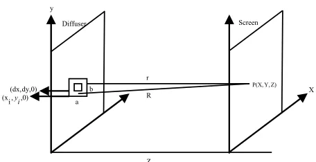
Suppose a grain of dimension (a, b) is located on the surface of the transparent diffuser (Figure 1), where its cen- ter having the coordinates (xi, yi, 0). The wave function

scattered from an element of dimensions (dxi, dyi, 0) lo-

cated at position (x, y, 0) and illuminating a point Pof coordinates (X, Y, Z) on a screen placed a distance apart from the diffuser is given by

 

0_ei wt kr_{d d}

a

x y r



  (1)

where a r₀ is the scattered amplitude per unit area from the diffuser,



 

2



2

2 2

r  X x  Yy Z (2) Let the grain under study is of dimensions a, b, and position (xi, yi, 0).



 

2



2

2 2

i i

R  X x  Y y Z (3) For X x and xi , and Yy and yi we get:









2

1 2

2

2 2

1 X x xi Y y yi

r R

R R

   

 _   _

(2)

y a Z dy,0) (dx, ) 0 , , i (x y_i

[image:2.595.58.286.81.198.2]

Diffuser b r R X Z) Y, P(X, Screen

Figure 1. Construction of the theoretical model. Using the Bernwlli inequality, one gets



1



n 1 n

1!

 

   for  1. Thus r can be written as



i





i



X x x r

R

 

 )

The integration of the wave amplitude given by Equa- tion (5), over the entire area of a grain pen

yi, 0) gives the resultant wave amplitude emitted from

an

Y y y R

R

  (5

sioned on (xi,

d reaching point Pon the screen as

  1 ₀ 2 2 1 _ 2 2

e i i e e d d

i i

a b

x y _{i wt kr} i

g a b

x y

a

A x y

r

   





_{ }

(6)

 

  0   0

0 0 2 2 0 1 2 2 e e e e i i i i i i i a a x y

kX x x kY y y

i i

R R

i wt kR i g a a x y a A kX kY

R _i _i

R R                 _ _ _ _         (7)    0 1 sin sin 2 2 e e 2 2

i i wt kR

i g

kXa kYb

a ab R R

A kXa kYb R R R              _ _  _ _                   (8)

Let now another type of grain of thickness



1



kZ z



1



k R

R

 

    

where 

R R

is the refracted index of used diffuser. Since



 the amplitude is considered to be constant. Thus the wave amplitude reaching the point P from the

gr

second ain type will be given by:

 

0 2

sin sin 2

eii ei wt kR

g

kXa kXb

a ab R

A   

           _      2 2 2 R kXa kXb R R R _{ }  _             (9) with

2 2 2 2 2

0 2 2

0

2

2 2 1 i i

i i

o

Xx Yy

R X Y Z Xx Yy R

R R

 

      _  

 

where 2 2 2 2

0

R  X Y Z

orem





. Using the binomial expan

sion the

-

1



2

1 n 1

1! 2!

n n nx

x  x

  

the higher term

 one gets

s



after excluding 0

0 0

.

Xxi Yyi

R R R

 

Let now an N × N number of grains of the first type iffuser, thus the resu ant wave

R



per unit area be resident on the d lt amplitude reaching the point P on the screen will be given by:

 

   

0

0 0 0 0

0 1

2 1 2 1

2 2

1 1

sin sin

eii

kXa kXb

a a

A  e 2 2

2 2

e e e e

i wt kR g

k a _N k k b _N k

i X i a l X i Y i b l Y

R R R R

l l

b R R

kXa kXb R R R x                 _ _  _ _                 



(10) i.e.

 0

1 2 0 1 2 0 1 2 sin sin 2 2 e e 2 2

1 e 1 e e

1 e 1 e

i i wt kR

i g

k aX bY _iN _iN

i R

i i

kXa kXb

a ab R R

 A kXa kXb R R R x x                          _ _  _ _                       (11)

where ₁

 

0

2

k _{a X}

R

  , and ₂

 

0

2

k _{b Y}

R

  .

Similarly for the second type of the grains of number er unit area, th ant wave reaching the point P will be given by:

N × N p e result

    0 1 2 0 1 2 3 2 2 2 2 2

1 e 1 e e e

1 e 1 e

wt kR

aX bY

k _iN _iN

i R i i i R R kXa kXb R R R x x                2 0 2 sin sin ei ei

g kXa kXb a ab A             _ _  _ _                        (12)

From Equations (11) and (12), it is seen that the phase difference between the two resultant waves



 2 1



is

given by:











0



_

_

0

1

kZ z k

aX bY R R       (13) Since 2 1 k aX bY R    





2 2

1 2 2 1 2cos 2

g g g g

I A  A  A A   1 (14)

(3)





2

2 1

2 1 cos

I  A _     2

0



 ₍₂₃₎

ere  (15)

For

0

i

Xx

R and 0

0

i

Yy R

 , it follows R

R R0 and



2 1











0 0

aX bY

R R .

1

kZ z  k

     

Setting Y = 0, and _sin 1 _sin 1

4 2    _           2

A can be

rewrite in the form

2 1 2

2 a a

A _{ } 

  0 1 sin 2 4 N b R         _ _          (16)

with

 

3 5 7

sin

3! 5! 7!

  

     ,

 

2 4 6

cos 1

2! 4! 6!

  

     

and



 

2



4

1 1

1 2 2

cos 1

2 3! 5!

N N

N  

 _{  } _ _

 

   (17)

2 2

2 0 ₄ 2 _cos 1

2

a ab N

A N R         _ _ _ _ _      

Thus the intensity can be written as

(18)





2 2 2 0 1 2 1

2 4 cos 1 cos 2

R

a ab N

I   N      

  _ _ _ _ __ _   _

(19) Setting

 

   

2 1 m

   , where









 



1



2 Z z aX

m c R    _ _    _{ }   _  _{ } _ and (19) 1 g

  , where g 2 2aX

c R



   

 (21)    _ _{ }

 

2

8 cos m

2 2

0 _{1 cos}

2

a ab Ng

I N R  _        _{ }  _   _ _ _ _ _     

In the forgoing derivation, monochromatic irradia- tion of the rough surface was considered. In the graph to follow, the rough surface will be assumed to be no

ing a symmetrical spectral line profile around (22)

para-

n-monochromatic having different spectral distribu-tion.

2.1. Gaussian Spectral Distribution

Assum 0

 

having a half width  and given by the

 

2 2

e

g   a₀   a_g   

to irradiate the rough surface of the target wh

 

2

g

a   

 and

_{ }

2

4ln 2

 



 .

The intensity on the screen might be given by:

I_G 

_

_ Ig

 

 d (24)

 

 2

0 2 2 e d G g R I

a   

2 2

2 0

8 a ab N cos Ng 1 cos m

            _ _ _      _ _       

_

Setting (25)

 

2 ₀ 2 ₂

4 ,

G g

a ab

c a N

R     _ _  





2 1 cos 1 cos

2 2 Ng Ng  _   _{ } _ _ _  _ _  

  ,   0x and

d dx.

























2

0 0

1 cos os

cos cos e d

G G

x

I C Ng x m x

x m x  x

c Ng          _         _



₍₂₆₎

The integration of (26) gives, with the following expression for the intensity dist g

N m

ribution

  







2 2 0 e m g N

I  N  

 (27) From (27) it is obvious that the intensity reaches its maximum as

4 0

1 2cos e cos

4

g

G CG _ m  _

     _   _  2 g

N _ m , and its minimum as



2 1



g

N  m , with m

min.

0,1, 2,3,

 . Considering

the

max.

G

I and IG

above conditions for maximum and minimum intensity in (27) and setting the obtained expressions for

, one obtains,

 





2 2 e 4 g N V   4 0

1 2 cos e

G

m

m_  

          _ _   (28)

2.2. Lorentzian Spectral Distribution

In this case it is assumed that a symmetrical spectral line profile around _ following a Lorentizian profile function,

 

2

 

2

0 0 2

0

1

L

a  a 

(4)

where

 

0 2

2

L

a 

 



The intensity distribution is

 

2

0 d

L o

I 

_

_ I a   (30)

















0

0 2

1 _dx₍₃₁₎ 1 cos Ng x 

   



1 cos

1

2

L L

I C m x

x



 



 

 _   _

 

 _ 

 



where ₄

 

2 0 2

L L

a ab

C a N

R





For ,

The L can be written as g

N m

n I





2





2

0 0

1 2cos e cos e

2

g

N m



L L g

I C m N

 

  _ _   



    

 

 

(32) From (32) it is obvious that the intensity is a maximum as 2N_g _ m,

with m0,1, 2,3

and its minimum as 

. Setting the above (3



2 1



g

N _ m , conditio

, ns in

2), one gets after determining I_L_max. and I_L_min. the following equation for the visibility





2

2 0

e

1 2 cos e

g

N

L _m

V

m



 

 

  

  

(33)

__

 

  

 

.

3. Results and Discussion

To illustrate the dependence of the visibility on the grain height (surface roughness, the spectral half width, and ions (28) and (33) are een the diffuser and the

ows the the density of the grains, Equat

computed for great distance betw

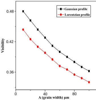
screen, this distance chosen in the computation to be equal 400 cm. The area of the diffuser is constant = 1 cm2_._{Figure 2}_{shows the obtained results between the}

visibility of the speckle patterns and the spectral half width. The calculation was carried out considering the grain height and height to be 106_{in cm}2 _{and 50}_μ_{m re-}

spectively. From the figure it is evident that the visibility of Gaussian distribution is greater than that obtained from Lorentzian one considers the same half width is due to the higher effective spectral band width in the Lor- entzian distribution which is larger than that in the case of the Gaussian one. The obtained behavior is in agreement with experimental data given in [6,11,12].

At a grain height of 10 μm, a spectral half width of 1012_{Hz and varying grain width, Equations (28) and (33)}

were computed to study the effect of the grain density on the visibility of speckle patterns. Figure 3 sh

0 40 80

0.36 0.42

0.48 Gaussian profile

Lorentzian profile

Vi

si

bi

li

ty

[image:4.595.337.506.84.259.2]

A (grain width) μm

Figure 2. The visibility of speckle patterns versus the spec-tral half width Δν with spectral line shape as a parameter. The results are obtained considering the grain density to be 106_{in cm}2_{, the grain height to be 50 µm.}

0 4 8 12

0.0 0.2 0.4

0.6 Gaussian profile

Lorentzian profile

Vi

si

bi

li

ty

(Hz)

[image:4.595.54.292.88.432.2]

x 1012

Figure 3. The visibility of the speckle patterns versus the grain width for the case of the Gaussian and Lorentzian profiles. The results are obtained for a grain height of 10 µm and spectral half width of 1012_Hz.

igher visibility of the speckle patterns. This behavior

igure 4 shows the dependence of the visibility of

dependence of the visibility of speckle patterns on the grain width in case of Gaussian and Lorentzian profiles. It is evident that the greater density of the grains yields h

can be interpreted by the following: By increasing the density, the randomization in difference between the in- terfering beam become smaller leading to increase the visibility.

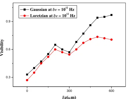
By keeping grain width equals 10μm and varying the grain height, Equations (28) and (33) were computed also to study the effect height on the visibility of the speckle patterns. F

speckle patterns on the grain height in case of Gaus- sian and Lorentzian spectral distributions at Δv = 1012_Hz. Figure 5 shows also the same, but for the case of Gaus- sian and Lorentzian spectral distributions at Δv = 1013_Hz.

[image:4.595.309.535.317.473.2]

(5)

0 300 0.3

0.6

600 0.9

V

isi

bi

li

ty

z(m)

[image:5.595.63.284.81.253.2]

Gaussian at 1012_Hz Loretzian at 1012_Hz

Figure 4. The visibility of the speckle patterns versus the grain height calculated for the case of Gaussian and Lor-entzian profiles of δυ = 1012_{Hz. The results are obtained for}

a grain density of 106_{in cm}2_.

0 20 40

0.02 0.04 0.06

60 0.08

Visib

ility

z(m)

Gaussian at  = Hz 1013 Lorentzian at = 1013 Hz

Figure 5. The visibility of the speckle patterns versus the grain height calculated for the case of Gaussian and Lor-entzian profiles of δυ = 1013_{Hz. The results are obtained for}

a grain density of 106_{in cm}2_.

rtially coherent e collimated light bject having dif- diation, the visibility of speckle patterns decreases. It is due to the inverse dependence of the degree of coherence of the light beam and its half width.

4. Experimental Verification

To verify the theoretical model an experiment as shown in Figure 6 was carried out using a pa

light obtained from a mercury lamp. Th illuminates a diffusely transmitting o

ferent surface roughnesses. The obtained speckle intensity distributions were captured by a webcam (digital camera). To find the relation between the speckle intensity fluctuation and the surface roughness, the surface roughnesses of these objects was precisely mechanically measured beforehand by suing a stylus instrument. Fig- ure 7 shows the obtained speckle pattern from partially

Object X

Webcam

2 P

1 P

3 L 1

L L₂

o

P

o

L S

[image:5.595.310.533.86.185.2]

F

[image:5.595.311.535.223.394.2]

Figure 6. The experimental setup used for the verification of the theoretical model.

Figure 7. The obtained speckle pattern from partially co-herent light.

coherent light.

By using software program (Image J), the value of the mean intensity I and the standard deviation σi of the

peckle pattern was obtained and substituted in the con-s

trast equation.

i

[image:5.595.63.283.311.477.2]

C I (34)

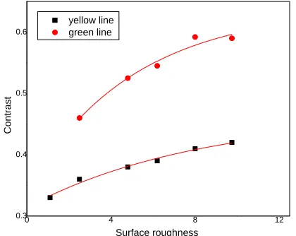
Figure 8 shows the dependence of the speckle patterns contrast on the surface roughness obtained from the two spectral lines of the Hg lamp (the

To increase the range of spectral se

el for a periodic rough sur- green and yellow line). half width, we used the tup in Figure 9. As we can see from the figure, the collimated light illuminates a diffraction grating D. The spectrum of Halogen lamp appears beyond the diffraction grating. By using a rectangle aperture, we can select bands with different widths. For each band width we repeat the previous experimental procedures. Figure 10

shows the dependence of the speckle patterns contrast on the surface roughness for different spectral half widths of values 2.9 × 1013_{Hz, 2.59 × 10}13_{Hz, 1.857 × 10}13_Hz,

1.295 × 1013_{Hz respectively.}

5. Conclusion

(6)

0 4 8 0.3

0.4 0.5

12 0.6

yellow line green line

Co

n

tr

a

s

t

[image:6.595.69.279.85.252.2]

Surface roughness

Figure 8. The relation between speckle patterns contrast and surface roughness.

Camera Video

Object D

C

RP L

[image:6.595.60.285.375.558.2]

S

Figure 9. The experimental setup used to increase the

of the spectral half width. range

0 5 10 15

0.00 0.05 0.10 0.15 0.20 0.25 0.30 0.35 0.40 0.45

Co

n

tr

ast

Roughness (m)

x1013Hz x1013Hz

x1013Hz x1013Hz

Figure 10. The relation between the speckle patterns con-trast and surface roughness with Δν = 2.9 × 1013_{Hz, 2.59 ×}

1013_{Hz, 1.857 × 10}13_{Hz, and 1.295 × 10}13_{Hz as a}

parame-ter.

tigated using partially coherent light. The general

[1] E. Archbuld, J. M. Burch and A. E. Ennos, “Recording of In-Plane Surfac e-Exposure Speckle

Photography,” No. 12, 1970, pp.

face was constructed. Depending on the new theoretical model, an equation for the visibility of speckle patterns is

nves i

behavior of the experimental results, which agree with

the published data, are in good agreement with the new theoretical model.

REFERENCES

e Displacement by Doubl Optica Acta, Vol. 17, 883-898. doi:10.1080/713818270

[2] K. R. Erf, “Speckle Metrology,” Chapter 4, Academic Press, New York, San Francisco, London, 1978.

[3] H. J. Tiziani, “Application of Speckling for In-Plane Vi- bration Analysis,” Optica Acta, Vol. 18, No. 12, 1971, pp. 891-902. doi:10.1080/713818406

[4] H. Fujii and T. Asakura, “Coherence Measurement of Quasi Monochromatic Thermal Light Using Speckle Pat- terns 1,” Optik, Vol. 39, 1973, pp. 99-117.

. 1, 1974, pp.

972, pp. 273-290.

[5] H. Fujii and T. Asakura, “Coherence Measurement of Quasi Monochromatic Thermal Light Using Speckle Pat- terns II,” Optik, Vol. 39, 1973, pp. 284-302.

[6] H. Fujji and T. Asakura, “A Contrast Variation of Image Speckle Intensity under Illumination of Partially Coherent Light,” Optics Communications, Vol. 12, No

32-38.

[7] T. Asakura, H. Fujii and K. Murata, “Measurement of Spatial Coherence Using Speckle Pattern,” Optica Acta, Vol. 19, No. 4, 1

doi:10.1080/713818561

[8] H. Fujiwara, T. Asakura and K. Murata, “Some Effects of Spatial and Temporal Coherence in Holograph

Acta, Vol. 17, No. 11, 19

y,” Optica 70, pp. 823-838.

doi:10.1080/713818257

[9] C. Parry, “Some Effects of Temporal Coherence on the First Order Statistics of Speckle,” Optica A

No. 10, 1974, pp. 763-772. doi:10.1080/713818852cta, Vol. 21,

. Li, s by Use [10] E. A. Guillemin, “The Mathematics of Circuit Analysis,”

John Wiley and Sons, New York, 1951, p. 530. [11] C. F. Cheng, C. X. Liu, N. Y. Zhang, T. Q. Jia, R. X

and Z. Z. Xu, “Absolute Measurement of Roughness and Lateral-Correlation Length of Random Surface

of the Simplified Model of Image-Speckle Contrast,” Ap- plied Optics, Vol. 41, No. 20, 2002, pp. 4148-4156. doi:10.1364/AO.41.004148