A cointegration and error correction approach to the determinants of inflation in India

Munich Personal RePEc Archive

A cointegration and error correction

approach to the determinants of inflation

in India

I, Sahadudheen

Pondicherry University

2012

Online at

https://mpra.ub.uni-muenchen.de/65561/

Determinants of Inflation in India

Sahadudheen I

Lecturer in Economics, Department of Economics,

Calicut University Centre, Kadmat, Lakshadweep, India [email protected]

Abstract

No doubt that the persistent rise in the price levels of commodities and services

adversely affects the economic performance. The goal of each and every Government is to

maintain low and relatively stable levels of inflation. Creeping or mild inflation can be

viewed as having favorable impacts on the economy; on the other hand zero inflation is

harmful to other sectors in the economy. The right level of inflation, is somewhere in the

middle. The study analyzed the major determinants of inflation in India extracting 54 time

series quarterly observations. The study employed Johansen-juselius cointegration

methodology to test for the existence of a long run relationship between the variables. The

cointegrating regression so far considers only the long-run property of the model, and does

not deal with the short-run dynamics explicitly. For this, the error correction from the long

run determinants of inflation is then used as a dynamic model to estimate the short run

determinants of inflation. The study concluded that the GDP and broad money have a

positive effect on the inflation in long run. On the other hand, interest rate and exchange rate

has a negative effect.The income coefficient is 0.37 and showing significant, implying that in

India, a one percent increase in income while others keep constant contributes 0.37%

increase in inflation. Similarly the money coefficient is 0.047 and showing significant,

implying that in India, one percent increase in money supply leads to a 5% increase in price

level.

Keywords: Wholesale price index, GDP, India, unit root, cointegration, Error correction

Introduction

Inflation is an important concept in the history of economic thought and can be

defined as a sustained rise in the general level of prices i.e. a persistent rise in the price levels

of commodities and services, leading to a fall in the currency’s purchasing power. High inflation is bad for the economy and it adversely affects economic performance. Even

moderate levels of inflation can distort investment and consumption decisions. Reducing

unemployment. The problem of inflation used to be confined to national boundaries, and was

caused by domestic money supply and price rises. In this era of globalization, the effect of

economic inflation crosses borders and percolates to both developing and developed nations.

Too much money in circulation, increases production costs, declines in exchange rates,

decreases in the availability of limited resources such as food or oil etc are the basic causes of

inflation. Inflation is a sign that an economy is growing, but excessive economic growth can

be detrimental as it can lead to hyperinflation as experienced, at the other extreme, an

economy with no inflation has essentially stagnated. The right level of economic growth, and

thus the right level of inflation, is somewhere in the middle. Creeping or mild inflation can be

viewed as having favorable impacts on the economy; on the other hand zero inflation is

harmful to other sectors in the economy with falling prices, profits, and employment. In

general, unpredicted running and galloping inflation are regarded has unprecedented effects

on an economy because it distort and disrupt the price mechanism, discourage investment and

saving, adversely effects fixed income group, creditors and ultimately leads to the breakdown

of morals.

Review of Literature

Gary G. Moser (1995) analyzed the dominant factors influencing inflation in Nigeria

by employing the cointegration and Error correction methods for the data ranges from 1960

to 1993. They used real income, broad money, annual rain fall and Naira-US dollar bilateral

exchange rate as their explanatory variables. They found that monetary expansion, driven

mainly by expansionary fiscal policies, explains to a large degree the inflationary process in

Nigeria. Other important factors were the devaluation of the naira and agro climatic

conditions.

Lim and Papi (1997) examined the major determinants of inflation in Turkey for the

ranging 1970 to 1995. The study employed Johansen Co integration technique and on the

basis of the result they concluded that money, wages, prices of exports and prices of imports

have positive influence on domestic price level where as exchange rate exerts inverse effect

on the domestic price level in Turkey.

Ilker Domaç (1998) investigated both the behavior and determinants of inflation in

Albania by applying co-integration and error-correction techniques to the inflation process.

They used Inflation, budget deficit, exchange rate depreciation, money growth and real GDP

as variables in his study. The results of the Granger Causality tests indicated that M1and the

exchange rate has an important predictive content for almost the entire individual items of the

run, inflation is positively related to both money supply and the exchange rate, while it is

negatively related to real income.

Kuijs (1998) investigated the major determinants of price level, output and exchange

rate in Nigeria using Vector Autoregressive (VAR) model. The study suggests that first lag of

prices, 3rd lag of prices, 1st lag of excess money supply and 1st lag of output gap are directly

related to price level where as 2nd lag of prices, 4th lag of exchange rate and output gap are

indirectly linked with price level in Nigeria.

Liu and Adedeji (2000) studied the determinants of inflation in the Islamic Republic

of Iran for data covering the period from 1989 to 1999. By applying Johansen co-integration

test and vector error correction model, they concluded that lag value of money supply,

monetary growth, four years previous expected rate of inflation are positively contributed

towards inflation while two years previous value of exchange premium is negatively

correlated with inflation.

Mosayed and Mohammad (2009) examined the determinants of inflation in Iran for

the data from 1971 to 2006. The study adopted Autoregressive and distributed lag model

(ARDL) and concluded that money supply, exchange rate, gross domestic product, change in

domestic prices and foreign prices, a variable that capture the effect of Iran or Iraq war are

the major determinants of inflation in Iran and all are positively contributing to the domestic

prices in Iran.

Abidemi and Malik (2010) analyzed simultaneous inter relationship between inflation

and its major determinants in Nigeria for the period from 1970 to 2007. The study adopted

Johansen co-integration methodology and error correction model (ECM) and conclude their

study revealing that growth rate of GDP, money supply, Imports, 1st lag of inflation and

interest rate are positively associated with inflation rate, while fiscal deficit and exchange rate

are indirectly associated to inflation.

Armstrong Dlamini and Tsidi Nxumalo (2011) used annual data from 1974 to 2000

and analyzed the determinants of inflation in Swaziland by employing the econometric

technique of cointegration and error correction model (ECM).They used real income,

nominal money supply, nominal interest rate, nominal exchange rates, nominal wages, and

South African consumer prices as explanatory variables and Swaziland consumer price index

as the dependent variable. They found that the impact of the money supply variable on

inflation is insignificant; suggesting that money supply growth in Swaziland does not accord

with normal behavioral expectations towards inflation. Interest rates seem to play no

rate has a significant long-run influence on the level of prices in Swaziland and the foreign

price as have a significant long run influence on the level of prices of Swaziland.

Data, Methodology and Empirical Results

In order to investigate the determinants of inflation in India, the following data are

used. The data used in this study are cumulated from various secondary sources. The variable

such as wholesale price index (WPI), broad money (M3), real gross domestic product

(GDPFC) and prime lending rate are collected from CMIE. The bilateral exchange rate

between dollar and rupee are collected from www.exchangerate.com. The data collected over

a period of 1996Q1 to 2009Q2. The WPI estimated 1993-94 constant prices, whereas GDPFC

is estimated on the basis of 1999-00 constant price and GDP and broad money are seasonally

adjusted.

To investigate the above issue the study uses the 54 quarterly observations from

1996Q1 to 2009Q2. The choice of sample period is due to capture short term dynamics of

inflation. In order to study the various determinants of inflation in India, we considered five

variables, namely WPI, real GDP, prime lending rate, broad money and bilateral exchange

rate. The statistical and time series properties of each and every variable are examined using

the conventional unit root test.

The study employs the econometric technique of cointegration and error correction

model (ECM) in order to estimate a more specific relationship between inflation and its

determinants. The ECM, as a tool of analysis, overcomes the problems of spurious regression

through the use of appropriate differenced variables in order to determine the short-term

adjustments in the model. Cointegration analysis on the other hand provides the potential

information about long term equilibrium relationship of the model.

The relationship between inflation and its key determinants is an important building

block in macro-economic theories and is a crucial component in the conduct of monetary

policy. The proper specification of the model is very important and constitutes primary step

for robust results to obtain. In all the countries the determinants of inflation are almost same,

only the difference is on their magnitude.

There are however, generally three functional forms dominating the literature:

linear-additive, log-linear and linear-no additive. There is general consensus that the log linear

version is the most appropriate functional form. We hypothesize that the fundamental

exchange rate. For estimation purposes, we use the logarithmic transformation of quarterly

data for the period 1996:01–2009:02. we specify the following equation, where all

variables except prime lending rate are expressed in logarithmic forms, is a random error term, and t is a quarterly time index.

Ln Pt=α+ lnYt + Rt+ фln εt + lnXt + t

P= wholesale price index (1993-94 base year prices)

Y= Nominal gross domestic product (1999-00 base year prices)

M= Broad money, R= Prime lending rate, X= rupee- dollar bilateral exchange rate

= error term

The first step of the strategy of our empirical analysis involves determining the order

of integration. Most time series are trended and therefore in most cases are nonstationary. The

problem with non stationary or trended data is that the standard OLS regression procedure

can easily lead to incorrect conclusion. A series of Augmented Dickey-Fuller unit root test is

performed to determine the order of integration of the variables.

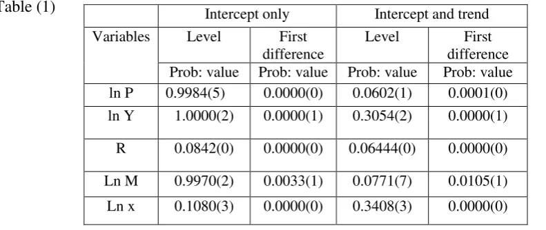
Table shows the ADF test results for both at the level and the first difference on

intercept and intercept and trend.

Table (1)

(Numbers in parenthesis are the number of lags)

The reported result in table reveals that the hypothesis of a unit root can’t be rejected

in all variables in levels. However, the hypothesis of a unit root is rejected in first differences

at 0.05 level of significant which indicates that all variables are integrated of degree one, I(1).

That means all the variables achieve stationarity only after first difference.

Intercept only Intercept and trend

Variables Level First

difference

Level First

difference

Prob: value Prob: value Prob: value Prob: value

ln P 0.9984(5) 0.0000(0) 0.0602(1) 0.0001(0)

ln Y 1.0000(2) 0.0000(1) 0.3054(2) 0.0000(1)

R 0.0842(0) 0.0000(0) 0.06444(0) 0.0000(0)

Ln M 0.9970(2) 0.0033(1) 0.0771(7) 0.0105(1)

The estimation of the equation by direct OLS gives the following integration

equation.

P=0.769524+0.031479yt-0.003224Rt+0.307648Mt-0.098304xt

^

(2.937358) (0.662551) (-1.458706) (8.804150) (-2.390108)

(0.0050) (0.5107) (0.1510) (0.000) (0.0207)

Adj R2= 0.994411 F= 2358.394 DW=1.165611

The estimated parameters of equation are in accordance with economic theory. Prime

lending rate and exchange rate have negative parameters while income and broad money has

positive coefficients. All coefficients are statistically significant at 0.05 % level except

income and prime lending rate. Here we have high R2 and t-values, but t is not white noise.

All the variables give the expected result, but the nonstationarity of variable biased the

previous estimation, and the low value of DW can be interpreted as sign of spurious

regression.

The criterion for selecting the lag length consist an important step. There are different

tests that would indicate the optimal number of lags. The study utilizes the SC criterion to

ensure sufficient power of the Johansen procedure.

The next step in our empirical analysis is to test for cointegration. Since the variables

are considered to be I(1), the cointegration method is appropriate to estimate the long run

demand for money. The concept of cointegration is that non-stationary time series are

cointegrated if a linear combination of these variables is stationary. The cointegration

requires the error term in the long-run relation to be stationary. Suppose there are two

variable Yt ad Xt and both Yt and Xt follows I (1) process, Still the linear combination

Ut=Yt - αXt is I (0). If so, both Yt and Xt are said to be cointegrated and a is the cointegrating

parameter. The maximum likelihood approach to test for cointegration is based on the

following system of equations

The number of independent cointegrating vector is equal to the rank of matrix π, If

rank of π = 0; then π is a null matrix and equation turns out to be a VAR model, whereas If

rank of π =1, there is one cointegrating vector and π xt-1 is an error correction term. Johansen

suggests that it can be done by testing the significance of characterizes roots of π.

t i t p

i i t

t x x

x     

  _







1

Johansen suggests two test statistics to test the null hypothesis that numbers of

characteristics roots are insignificantly different from unity.

λi = estimated characteristic roots or Eigen values

T = the number of usable observations

λ trace test the null hypothesis

r = 0 against the alternative of r > 0

λmax test the null hypothesis

r = 0 against the alternative of r = 1

The theory asserts that there exists a linear combination of this non-stationary that is

stationary. Solving for the error term, we can rewrite the relation as

t=α- lnYt - Rt -фln εt - lnXt

Since { t} must be stationary, it follows that the linear combination of integrated variables

given by the right hand side of must also be stationary.

Cointegration test result

Unrestricted cointegration Rank test (Trace)

Null hypothesis Eigen Value Trace statistics 5 percent critical value Porb.**

r=0* 0.576467 102.6474 69.81889 0.0000

r≤1*

0.467886 57.97292 47.85613 0.0042

r≤β 0.233837 25.16622 29.79707 0.1556

r≤γ 0.148988 11.31545 15.49471 0.1928

r≤4 0.054722 2.926370 3.841466 0.0871

Unrestricted cointegration Rank test (Maximum Eigenvalue)

Null hypothesis) Eigen Value Max-Eigenvalue 5 percent critical value Porb.**

r=0* 0.576467 44.67449 33.87687 0.0018

r≤1* 0.467886 32.80671 27.58434 0.0097

r≤β 0.233837 13.85076 21.13162 0.3774

r≤γ 0.148988 8.389084 14.26460 0.3405

r≤4 0.054722 2.926370 3.841466 0.0871

(* denotes the rejection of the hypothesis at the 0.05 level. And _** are Mackinnon-Hauge-Michelis (1999) p-values.)

The above table shows that the null hypothesis of no cointegration is rejected at the

conventional level (0.05) and the study conclude that there exists a relationship among the )

ˆ

1 ln( )

1 , (

)

ˆ

1 ( ln )

(

1 max

1

 



 

 

 





r i n

r i trace

T r

r T r

 

proposed variables in the long run. Trace test and Eigen value test indicates that there are two

cointegrationg vector.

The normalized cointegration equation is depicted in above table which reveals that

the income and money has a positive effect on inflation. On the other hand, prime lending

rate and exchange rate has a negative. The income coefficient is 0.37 and showing

significant, implying that in India, a one percent increase in income while others keep

constant contributes 0.37% increase in inflation. Similarly the money coefficient is 0.047 and

showing significant, implying that in India, one percent increase in money supply leads to a

5% increase in price level. Interest rate and exchange rate carries expected negative and

significant coefficient.

By specifying the long run determinants of inflation in an error correction model, the

short run as well as the long run effects of all right hand side variables in equation are

estimated in one step, which is a major advantage that error correction modeling has in

comparison to other estimation.

The dynamic relationship includes the lagged value of the residual from the

cointegrating regression ( t-1) in addition to the first difference of variables which appear in

the right hand side of the long run relationship (Y, M, R and X). The inclusion of the

variables from the long run relationship would capture short run dynamics.

The ECM simply defined as

xt t t t t t t mt t t t t t t Rt t t t t t t yt t t t t t t pt t t t t t t X M R Y P x X X M R Y P m M X M R Y P r R X M R Y P y Y X M R Y P p P                                                                                                     ) ( ) ( ) ( ) ( ) ( 1 1 1 1 1 1 1 1 1 1 1 1 1 1 1 1 1 1 1 1 1 1 1 1 1

Where, the elements of t s are white noise errors and s are speed of adjustment

parameters and α , , ,ф and are short run parameters. All the variable in the ECε are

stationary, and therefore, the ECM has no problem of spurious regression. Normalized cointegration coefficients

lnP lnY R lnM lnx

1.0000 0.376811

Error correction D(P) D(Y) D(R) D(M) D(X)

Coint Eq1 0.310190 -1.327206 2.406123 -0.041910 -0.322688

Standard error (0.09888) (0.24730) (3.76831) (0.11202) (0.31411)

t statistics [-3.13701] [ 5.36680] [-0.63851] [ 0.37413] [ 1.02731]

The above table shows the speed of adjustment coefficients, which reveals that only

two variables are adjusting. The adjustment coefficient on cointegration equation 1 for the

GDP is negative. The adjustment coefficient for broad money and exchange rate are showing

negative, as it should be, but both adjusting coefficient are showing insignificant. Similarly

adjustment coefficient for prime lending rate is showing positive, as it should be. But the

estimated error correction model enjoys a very low goodness of fit (R2=0.248572, adj R2

=0.0178382). The empirical study is performed by using PC version of Eviews 6.0.

Conclusion

The study used five variables extracting 54 quarterly observations from 1996Q1 to

2009Q2. Since all the variables have unit root at levels the study utilizes Johansen-juselius

cointegration analysis to test for the existence of a long run relationship between the

variables. The cointegrating regression so far considers only the long-run property of the

model, and does not deal with the short-run dynamics explicitly. For this, the error correction

from the long run determinants o0f inflation is then used as a dynamic model to estimate the

short run determinants of inflation. Both the trace test and Eigen value test indicates that there

are two cointegrationg vector. The study concluded that the GDP and broad money have a

positive effect on the inflation in long run. On the other hand, interest rate and exchange rate

has a negative effect. All variables carry expected result. The income coefficient is 0.37 and

showing significant, implying that in India, a one percent increase in income while others

keep constant contributes 0.37% increase in inflation. Similarly the money coefficient is

0.047 and showing significant, implying that in India, one percent increase in money supply

leads to a 5% increase in price level.

References

1. Abidemi, O. I. and εalik, S. A. A. (β010) ‘Analysis of Inflation and its determinant in

Nigeria’, Pakistan Journal of Social Sciences, 7(β), 97-100.

2. Cheng Hoon Lim and δaura Papi(1997) ‘An Econometric Analysis of the

Determinants of Inflation in Turkey’, IεF working paper WP/97/170

4. Dimitorios Asteriou (β010) ‘Applied Econometrics, A εodern Approach Using

Eviews And εicrofit’, Palgrave εacmillan Publication, β006.

5. Gary G. εoser (1995) ‘The εain Determinants of Inflation in Nigeria’ IεF Staff

Papers, Vol. 42, No. 2 (June 1995)

6. Ilker Domaç (1998) ‘The main determinants of inflation in Albania’, World Bank

Policy Research Working Paper No. 1930

7. Juan J. Dolado a, Jesús Gonzalo and Francesc εarmol (1999) ‘Cointegration’,

February, pp 12-19

8. δim, C. H. and Papi, δ. (1997). ‘An Econometric Analysis of the determinants of

Inflation in Turkey’, IεF Working paper no. 170, 1 – 32.

9. δiu, O. and Adedeji, O. S. (β000) ‘Determinants of Inflation in the Islamic Republic

of Iran: A εacroeconomic analysis’, IεF Working paper 1β7, 1 – 28.

10.εosayed, P and εohammad, R. (β009) ‘Sources of Inflation in Iran: An application

of the real approach’, International Journal of Applied Econometrics and Quantitative