Estimation of a system of national accounts: implementation with mathematica

Munich Personal RePEc Archive

Estimation of a System of National

Accounts: Implementation with

Mathematica

Temel, Tugrul

Development Research Institute (IVO), Tilburg University

8 December 2011

Estimation of a System of National Accounts:

Implementation with

Mathematica

Tugrul Temel

Development Research Institute (IVO)

Tilburg University, Tilburg

The Netherlands

[email protected]

December 15, 2011

Abstract

This study implementsMathematica to estimate a system of national accounts. The esti-mation methods applied are portrayed in Danilov and Magnus (2008), including the Bayesian estimation, restricted and unrestricted least-squares estimation and best linear unbiased esti-mation. Operationalizing these methods in the Mathematica environment is the main contri-bution of the current study. In light of the United Nations’ e¤orts aimed to standardize across countries the compilation of national accounts, theMathematica codes developed here should provide an important tool both for the estimation of unrealized or unavailable national accounts data and for conducting cross-country and within-country macroeconomic policy analysis.

Key words: System of national accounts; Social Accounting Matrix; Bayesian estimation; Least-squares estimation; Best linear unbiased estimation; Linear programming

———————————————–

1

Introduction

This study implements Mathematica to estimate a system of national accounts (SNA). The es-timation methods applied are portrayed in Danilov and Magnus (2008), including the Bayesian estimation, restricted and unrestricted least-squares estimation and best linear unbiased estima-tion. Operationalizing these methods in the Mathematica environment is the main contribution of the current study. In light of the United Nations’ e¤orts aimed to standardize across countries the compilation of national accounts, the Mathematica codes developed here should provide an important tool both for the estimation of unrealized or unavailable national accounts data and for conducting cross-country and within-country macroeconomic policy analysis. TheMathematica

codes should bene…t the most statistics organizations responsible for the compilation and updating of national accounts and policy-making bodies drawing on national accounts data.

The study is organized into …ve sections. Following the Introduction, Section 2 formulates a data estimation problem drawing on an example system of national accounts. Section 3 describes four estimation methods. Section 4 describes the implementation of the computational algorithm developed and presents the estimations concerning the example SNA. Finally, Section 5 concludes the paper with some remarks on the e¢ciency ofMathematicafor solving large linear systems.

2

An example system of national accounts

2.1

Set-up

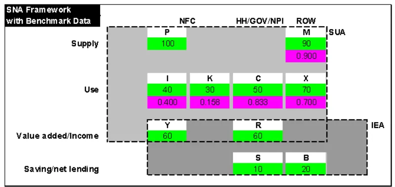
Consider an example SNA illustrated in Figure 1. The SNA consists of two sub-accounts: supply and use accounts (SUA) and integrated economic accounts (IEA), and is fully characterized by 10 variables. Given a benchmark (or reference) SNA at periodt= 0 and 4 variables known with precision at period t = 1 (see Figure 2), the goal is to estimate the remaining 6 variables for

t= 1. To do that, we utilize two additional pieces of information. First, …ve indicator ratios are constructed drawing on expert knowledge about the long-run behavior of the economy concerned. Second, six linear restrictions (or identities) are introduced using macro-accounting relations among the variables in the SNA (see Figure 3).

Below, we describe the set-up using mathematical notations.

Notations

~

xt

i denotes timetvalue of the i

th_{variable withi= 1;2; :::;~nand t= 0;1:} ~

xt_{= (~x}t

1;x~t2; :::;x~nt~)0 is a column vector ofn~ variables at timet:

fk(~xt) = 0 de…nes thekthidentity as a function ofx~t:

Assumptions 1)x~t

i N( t

i; 2i)for alli:

2)R0ij =R1ijform~1prior indicator ratios whereRij0 =

~

x0

i

~

x0

j is a prior indicator ratio evaluated using benchmark data. Reliability levels and reliability coe¢cients for p~ data observations made att= 1and form~1indicator ratios are set using prior information about the quality of available data: {Fixed = 0, Strong = 0.01, High = 0.03, Medium = 0.06, Low = 0.12, Poor = 0.24}.

Available data, priors and restrictions

1) Att= 0, benchmark data are available onn~ variables: ~x0= (~x01;x~02; :::;x~0n~)0: 2) Att= 1, data are available onp~variables: (~x11;x~12; :::;x~1p~)0 withp <~ n:~ 3) Att= 1,m~1 indicator ratios are available

4) Att= 0;1;linear restrictionsfk(~xt) = 0hold for allk= 1;2; :::;m~2

Technically speaking, the objective is to estimate the posterior mean and variance of variables in vectorx~1_{;on some of which data are available with precisions (p~), on some prior indicator ratios} are available with precisions (m~1), and on some prior information is available with precisions (m~2).

2.2

Data and prior information

In what follows, we translate the data and information given in Figures 1-3 into mathematical format so that one can link the example SNA to the estimation methods formally presented in the following sections. Suppose that at timet= 0a benchmark (or reference) data set is available for a vector ofn~= 10latent variables, denoted by:

~

x0 (~x0₁;x~0₂;x~0₃;x~0₄;x~0₅;x~0₆;x~0₇;x~₈0;x~0₉;x~0₁₀)0

= (P0; M0; I0; K0; X0; C0; Y0; R0; S0; B0)0

= (100;90;40;30;70;50;60;60;10;20)0_:

At timet= 1, data are available only for 4 variables(~p= 4):

(~x11;x~12;x~14;x~15)0 (P1; M1; K1; X1)0

= (107:12;93:64;32:14;74:98)0

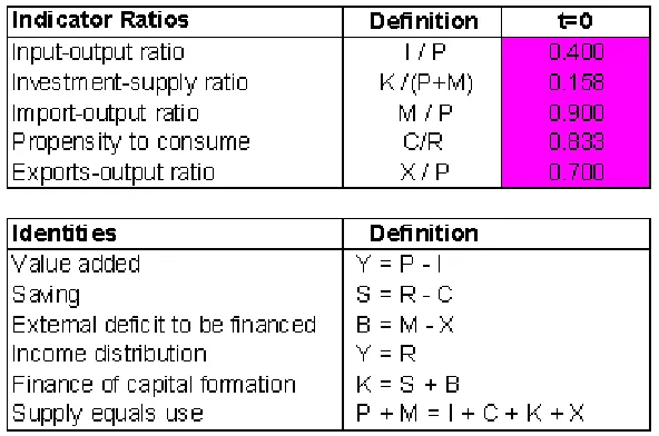
Furthermore, the benckmark values of the following 5 prior indicator ratios( ~m1= 5)are assumed to remain the same over the period fromt= 0tot= 1, implying that the economy has been in the state of equilibrium during that period.

(I

0

P0) =

40 100 = 0:4 ( K

0

P0_+M0) =

30

190 = 0:158 (M

0

P0) =

90 100 = 0:9 (C

0

R0) =

50

60 = 0:833 (X

0

P0) =

As a last piece of information, we assume that the following 6 linear restrictions ( ~m2 = 6) hold across allt, re‡ecting the basic macro-accounting relations among the~nvariables:

Yt _Pt_+It ₀

St Rt+Ct 0

Bt Mt+Xt 0

Yt Rt 0

Kt St Bt 0

Pt+Mt It Ct Kt Xt 0:

2.3

The system of linear equations

Data available(~p= 4)att= 1are expressed as:

~

D1x~1 = d~1 where

~

D1 =

2 6 6 4

1 0 0 0 0 0 0 0 0 0 0 1 0 0 0 0 0 0 0 0 0 0 0 1 0 0 0 0 0 0 0 0 0 0 1 0 0 0 0 0

3 7 7 5

~

x1 = (P1; M1; I1; K1; X1; C1; Y1; R1; S1; B1)0

~

d1 = (107:12;93:64;32:14;74:98)0

The "linearized" indicator ratios( ~m1= 5)assumed to hold for allt are expressed as

~

A1x~t ~h1 where

~

A1 =

2 6 6 6 6 4

0:4 0 1 0 0 0 0 0 0 0 0:158 0:158 0 1 0 0 0 0 0 0 0:9 1 0 0 0 0 0 0 0 0 0 0 0 0 0 1 0 0:833 0 0 0:7 0 0 0 1 0 0 0 0 0

3 7 7 7 7 5

~

xt _{= (P}t_{; M}t_{; I}t_{; K}t_{; X}t_{; C}t_{; Y}t_{; R}t_{; S}t_{; B}t₎0

~

h1 = (0;0;0;0;0)0

The linear restrictions( ~m2= 6)are:

~

A2x~t ~h2 for allt, where

~

A2 =

2 6 6 6 6 6 6 4

1 0 1 0 0 0 1 0 0 0 0 0 0 0 0 1 0 1 1 0 0 1 0 0 1 0 0 0 0 1 0 0 0 0 0 0 1 1 0 0 0 0 0 1 0 0 0 0 1 1 1 1 1 1 1 1 0 0 0 0

3 7 7 7 7 7 7 5

~

xt = (Pt; Mt; It; Kt; Xt; Ct; Yt; Rt; St; Bt)0

~

2.4

The modi…ed system of linear equations

Owing to the numerator(Pt_+Mt_{)of the2}nd_{indicator ratio above, we de…ne a composite variable}

Zt _(Pt_+Mt_{)where Z}0 _{= 190 and Z}1 _{= 200:76: The introduction of this composite variable} requires some modi…cations in the linear system described in section (2.2). The …rst modi…cation takes place inD~1x~1= ~d1as follows:

D1x1 = d1 where

D1 =

2 6 6 6 6 4

1 0 0 0 0 0 0 0 0 0 0 0 1 0 0 0 0 0 0 0 0 0 0 0 0 1 0 0 0 0 0 0 0 0 0 0 0 1 0 0 0 0 0 0 0 0 0 0 0 0 0 0 0 0 1

3 7 7 7 7 5

x1 = (P1; M1; I1; K1; X1; C1; Y1; R1; S1; B1; Z1)0

d1 = (107:12;93:64;32:14;74:98;200:76)0 The second modi…cation takes place inA~1x~t ~h1as follows:

A1xt h1 where

A1 =

2 6 6 6 6 4

0:4 0 1 0 0 0 0 0 0 0 0 0 0 0 1 0 0 0 0 0 0 0:158 0:9 1 0 0 0 0 0 0 0 0 0 0 0 0 0 0 1 0 0:833 0 0 0 0:7 0 0 0 1 0 0 0 0 0 0

3 7 7 7 7 5

xt _{= (P}t_{; M}t_{; I}t_{; K}t_{; X}t_{; C}t_{; Y}t_{; R}t_{; S}t_{; B}t_{; Z}t₎0

h1 = (0;0;0;0;0)0

The third modi…cation takes place inA~2x~t h~2 by introducing the new identityZt (Pt+Mt) :

A2xt h2 where

A2 =

2 6 6 6 6 6 6 6 6 4

1 0 1 0 0 0 1 0 0 0 0 0 0 0 0 0 1 0 1 1 0 0 0 1 0 0 1 0 0 0 0 1 0 0 0 0 0 0 0 1 1 0 0 0 0 0 0 1 0 0 0 0 1 1 0 1 1 1 1 1 1 0 0 0 0 0 1 1 0 0 0 0 0 0 0 0 1

3 7 7 7 7 7 7 7 7 5

xt (Pt; Mt; It; Kt; Xt; Ct; Yt; Rt; St; Bt; Zt)0

Our goal is to solve the following system of equations using the estimation methods introduced in Section 3.

D1x1 = d1 with d1jxt Np(D1xt; 1)

A1x1 h1with A1 Nm1(h1; H1)

A2x1 = h2with A2 Nm2(h2; H2)(asy.)

where p = (~p+ 1) = 5

n = (~n+ 1) = 11

m1 = m~1= 5

m2 = ( ~m2+ 1) = 7

m = (m1+m2) = 12

3

Estimation Methods

The reader is referred to Danilov and Magnus (2008) for a detailed description of the estimation problems stated below. Although they are equivalent and all yield the same estimations, the performance of their computerized solution algorithms di¤er substantially depending on the size and sparsitiy of the linear system concerned.

3.1

Bayesian estimation

Assume (i)d1jx1 Np(D1x1; 1)whereD1;(p;n)has full row-rank and 1is positive de…nite (hence non-singular); (ii) Ax1 Nm(h; H)where A= (A1 :A2), a column vector h= (h1; h2); a block diagonal matrixH = (H1; H2)with H1 associated with A1 and H2 withA2; (iii) A has full row-rank and H may be singular. If m < n, letL be a semi-orthogonal (n; n m) matrix such that

LT_{L = I}

n m and AL = 0; and assume that the identi…ability condition r(A) +r(D1L) = n is satis…ed. Then the posterior distribution ofx1is given byx1jd1 Nn( ; V)with

V = A+HA+0 A+HA+0D10 01D1A+HA+

0

+CKC0

= A+h (A+HA+0+CK)D₁0 ₀1(D1A+h d1) where A+ = A0(AA0) 1 "the Moore-Penrose inverse"

0 = 1+D1A+HA+

0 D01

C = In A+HA+

0

D0_{1 0}1D1

K = L(L

0

D0_{1 0}1D1L) 1L

0

if m < n (Lemma A2)

0 ifm=n (Lemma A1)

3.2

Restricted least-squares estimation

For estimations in large systems, the least-squares method works better compared to the Bayesian estimation method (Theorem 1). The Bayesian problem above can be equivalently formulated as a restricted least-squares problem:

Minimize

x (d Dx)

0 1_{(d Dx) subject to A} 2x=h2

where d = Dx+

d j x Np+m1(Dx; )

Np+m1(0; )and

d = d1

h1 ; D=

D1

A1 ; =

1 0

0 H1 :

From Theorem 36 in Magnus and Neudecker (1999) (p.233), the general solution,x, to this mini-mization problem is:

x = x0+N+A

0

2(A2N+A

0

2)+(h2 A2x0) + (In N N+)q

wherex0 = N+D

0 ₁ d N = D0 1D+A0₂A2

q = an arbirary vector Computexby using:

d= 2 6 6 6 6 6 6 6 6 6 6 6 6 6 6 4

107:12 93:64 32:14 74:98 190 0 0 0 0 0 3 7 7 7 7 7 7 7 7 7 7 7 7 7 7 5

; D=

2 6 6 6 6 6 6 6 6 6 6 6 6 6 6 4

1 0 0 0 0 0 0 0 0 0 0 0 1 0 0 0 0 0 0 0 0 0 0 0 0 1 0 0 0 0 0 0 0 0 0 0 0 1 0 0 0 0 0 0 0 0 0 0 0 0 0 0 0 0 1 0:4 0 1 0 0 0 0 0 0 0 0 0 0 0 1 0 0 0 0 0 0 0:16 0:9 1 0 0 0 0 0 0 0 0 0 0 0 0 0 0 1 0 0:8 0 0 0 0:7 0 0 0 1 0 0 0 0 0 0

3 7 7 7 7 7 7 7 7 7 7 7 7 7 7 5 = 2 6 6 6 6 6 6 6 6 6 6 6 6 6 6 4

41:3 0 0 0 0 0 0 0 0 0 0 7:9 0 0 0 0 0 0 0 0 0 0 14:9 0 0 0 0 0 0 0 0 0 0 5:1 0 0 0 0 0 0 0 0 0 0 64:5 0 0 0 0 0 0 0 0 0 0 1:4 0 0 0 0 0 0 0 0 0 0 0:8 0 0 0 0 0 0 0 0 0 0 29:2 0 0 0 0 0 0 0 0 0 0 35:8 0 0 0 0 0 0 0 0 0 0 17:6

A2=

2 6 6 6 6 6 6 4

1 0 1 0 0 0 1 0 0 0 0 0 1 0 0 1 0 0 0 0 1 0 0 0 0 0 0 0 1 1 0 0 0 0 0 0 1 0 0 0 0 1 1 0 1 1 1 1 1 1 0 0 0 0 0 1 1 0 0 0 0 0 0 0 0 1

3 7 7 7 7 7 7 5

3.3

Unrestricted least-squares estimation

Alternatively, the solution of the following unrestricted minimization problem is also identical to that of the Bayesian estimation ofx:

Minimize d Dx

h2 A2x

0

+DD0 A2D0

DA02

A2A02

!

d Dx h2 A2x

whered = d1

h1 ; D=

D1

A1 ; =

1 0

0 H1

3.4

Best linear unbiased estimation

Best linear unbiased estimation (BLUE) is an alternative method that leads to the same results as restricted least-squares method. Consider the regression model:

Minimize(d Dx)0 1(d Dx) subject to: A2x=h2

wherexis a vector of parameters to be estimated. The BLUE estimator ofxis given by:

x = G 1D0 1d+G 1A0₂(A2G 1A02) 1(h2 A2G 1D

0 ₁ d)

with varianceV = G 1 G 1A02(A2G 1A02) 1A2G 1 where G = D0 1D+A0₂A2

d = d1

h1 ; D=

D1

A1 ; =

1 0

0 H1

4

Implementation

4.1

Algorithm

Mathematica codes for each one of the estimation problems above have been developed using

Mathematica8.0. The implementation algorithm applies the following steps. STEP 1: Testing the rank condition: r(A) +r(D1L) =n:

This condition is necessary and su¢cient for the existence of a solution. In our example, the rank of A is 11, which is also equal to the number of variables in the system; that is,

STEP 2: Creating a system of linearly independent equations

Having applied the Gram-Schmidt method to the set of 7 identities, we …nd out that 6 identities (excludingZt _Pt_+Mt_{) are linearly dependent. Hence, dropping any one of the}

6 identities fromAleads to a system of 11 equations, which then implies that the system at hand is fully identi…ed with rank 11. Here is a sketch of how to perform this task.

(1) Determine the rank ofAwith dimension of(m; n) = (12;11)where m=the number of rows,n=the number of columns.

(2)rk(A) = 11implies that one of the equations is redundant, which needs to be eliminated fromAfor the unique solution to exist.

(3) Apply Gram-Schmidt process to identify the linearly dependent equation. The process would generate a zero row for the dependent equation. Since dependency is a property of a group of equations, not a property of a single equation, Gram-Schmidt process results in a di¤erent dependent equation every time we change the order of rows in A. Thus, we obtain 6 alternative systems, each of which has 11 equations and has a non-zero determinant. (Note that a non-zero determinant implies that the system of equations concerned comprises a linearly independent set.)

(4) There are 6 non-zero determinants. This implies that the …nal Bayesian estimation should be performed for each one of 6 systems separately and the one that minimizes posterior standard deviation should be used in the …nal analysis.

STEP 3: Constructing a variance-covariance matrix

Due to the elimination of the dependent equation(s) fromA, necessary adjustments are made in the vectorhand the variance-covariance matrixH.

STEP 4: Introducing reliability levels and reliability parameters to create an adjusted variance-covariance matrix

The Bayesian data estimation approach allows for the deviation from the "true" values of the benchmark values of the indicator ratios and the data observations. Reliability levels assigned to each ratio and each one of the 4 observations imply that the "true" values are most likely to lie within the con…dence intervals implied by the reliability levels. The concept of reliability bridges the gap between the "true" and "observed" values of a variable. We set reliability levels as: {Fixed (F), Strong (S), High (H), Medium (M), Low (L), Poor (P)}, with arbitrary reliability coe¢cients of {0, 0.01, 0.03, 0.06, 0.12, 0.24}, respectively. Coe¢cient of variation, de…ned by the ratio of standard error to mean, represents reliability coe¢cient. Given the reliability coe¢cient and the mean value at t = 0 of the variable of interest (see Table 1), we calculate prior standard error of that variable. In the rest of the paper, matrix notation is used for convenience. Estimate the variance-covariance matrices ( 1; H) for time t = 1 observations and for the indicator ratios, respectively. In the estimation of 1associated with

Table 1

V ariable R coef f M ean P rior s:e: P rior var:

P1 _{M=0.06 107.12 6.43 41.3}

M1 _{H=0.03 93.64 2.81 7.9}

K1 _{L=0.12 32.14 3.86 14.9}

X1 _{H=0.03 74.98 2.25 5.1}

Z1 _{MH=0.04 200.76 8.03 64.5}

Consider, for example, P1, which is assumed to be observed at the Medium level, with a corresponding reliability coe¢cient of 0.06. Applying the de…nition of coe¢cient of variation

= seP1

M ean of P1 would then yield prior standard errorse_P1 = 0:06 107:12 = 6:427 2. Thus,

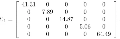
the prior variance is41:3. This operation yields

1= 2 6 6 6 6 4

41:31 0 0 0 0 0 7:89 0 0 0 0 0 14:87 0 0 0 0 0 5:06 0 0 0 0 0 64:49

3 7 7 7 7 5 :

The estimation ofH associated withA is a bit complex. H1 corresponding to the indicator ratios is a (5,5) diagonal matrix, elements of which are 2

ijBij2, whereasH2 corresponding to the identities is a (6,6) zero matrix:Table 2 shows how to deriveH1:

Table 2

Indicator Ratios

R coef f

E(xti

xt j)

=rij

P rior s:e:

P rior var ( 2

ij) B2ij 2ijBij2 xt

3

xt

1 =

It

Pt H=0.03 0.4 0.012 0.00014 10000 1.4

xt4

xt

11 =

Kt

Zt H=0.03 0.16 0.005 0.00002 36076 0.8

xt

2

xt

1 =

Mt

Pt M=0.06 0.9 0.05 0.0029 10000 29

xt

6

xt

8 =

Ct

Rt L=0.12 0.83 0.1 0.0099 3612 36

xt5

xt

1 =

Xt

Pt M=0.06 0.7 0.04 0.0018 10000 18

The ratios are assumed to be distributed as(xti

xt j)

Nm2(rij;

2

ij), while the linearized ratios as(xt

i rijxtj) Nm2(0;

2

ijBij2). The benchmark datax0 are used to calculate:

Bij =

8 > < > : r2 ij

(1+r2

ij)rijxi+

1 (1+r2

ij)

xj if bothxi andxj are available xi

rij if onlyxi is available

xj if onlyxj is available

9 > = > ;

Sincem=n, Lemma A1 of Theorem 1 applies. The full system is characterized by(D1; d1; 1; A; h; H), where

D1=

2 6 6 6 6 4

1 0 0 0 0 0 0 0 0 0 0 0 1 0 0 0 0 0 0 0 0 0 0 0 0 1 0 0 0 0 0 0 0 0 0 0 0 1 0 0 0 0 0 0 0 0 0 0 0 0 0 0 0 0 1

d1= 2 6 6 6 6 4

107:12 93:64 32:14 74:98 190 3 7 7 7 7 5

; 1=

2 6 6 6 6 4

41:3 0 0 0 0 0 7:9 0 0 0 0 0 14:9 0 0 0 0 0 5:1 0 0 0 0 0 64:5

3 7 7 7 7 5 A= 2 6 6 6 6 6 6 6 6 6 6 6 6 6 6 6 6 4

0:4 0 1 0 0 0 0 0 0 0 0 0 0 0 1 0 0 0 0 0 0 0:16 0:9 1 0 0 0 0 0 0 0 0 0 0 0 0 0 0 1 0 0:83 0 0 0 0:7 0 0 0 1 0 0 0 0 0 0

1 0 1 0 0 0 1 0 0 0 0

0 1 0 0 1 0 0 0 0 1 0

0 0 0 0 0 0 1 1 0 0 0

0 0 0 1 0 0 0 0 1 1 0

1 1 1 1 1 1 0 0 0 0 0

1 1 0 0 0 0 0 0 0 0 1

3 7 7 7 7 7 7 7 7 7 7 7 7 7 7 7 7 5 h= 2 6 6 6 6 6 6 6 6 6 6 6 6 6 6 6 6 4 0 0 0 0 0 0 0 0 0 0 0 3 7 7 7 7 7 7 7 7 7 7 7 7 7 7 7 7 5

; H=

2 6 6 6 6 6 6 6 6 6 6 6 6 6 6 6 6 4

1:4 0 0 0 0 0 0 0 0 0 0 0 0:8 0 0 0 0 0 0 0 0 0 0 0 29:2 0 0 0 0 0 0 0 0 0 0 0 35:8 0 0 0 0 0 0 0 0 0 0 0 17:6 0 0 0 0 0 0 0 0 0 0 0 0 0 0 0 0 0 0 0 0 0 0 0 0 0 0 0 0 0 0 0 0 0 0 0 0 0 0 0 0 0 0 0 0 0 0 0 0 0 0 0 0 0 0 0 0 0 0 0 0 0 0 0 0 0 0 0 0 0 0 0 0

3 7 7 7 7 7 7 7 7 7 7 7 7 7 7 7 7 5

4.2

Estimation of the example SNA

The estimation results and the Mathematica codes generating these results are given in Table 3.

5

Concluding remarks

Four estimation methods have been operationalized usingMathematica 8.0. An example system of national accounts has been used for illustrative purposes. We have developed a genericMathematica

code (translated to C++) for each one of the 4 estimation problems. The codes are applied to very large systems. The power ofMathematica (C++)remains to be compared with the SNAER program of Danilov and Magnus (2008).

References

[1] Abadir, K. M., and Magnus, J. R. (2005). Matrix Algebra. Econometric Exercises 1. Cambridge, UK: Cambridge University Press.

[2] Danilov, D., and Magnus, J.R. (2007). Some equivalences in linear estimation. On-line: http://cdata4.uvt.nl/website…les/magnus/paper77b.pdf.

[3] Danilov, D., and Magnus, J. R. (2008). On the estimation of a large sparse Bayesian system: The Snaer program. Computational Statistics & Data Analysis, 52(9), 4203-4224.

[4] Danilov, D., and Magnus, J. R. (2005). Least-squares estimation in large sparse systems. Work in progress.

[5] Golub, Loan. (1983). Matrix Computations.

[6] Huang, C. J., and Crooke, P.S. (1997). Mathematics and Mathematica for economists. Oxford, UK: Blackwell Publishers.

[7] Jing Xiao , Lan Liu , Lirong Xia and Tao Jiang. (2007). Fast Elimination of Redundant Linear Equations and Reconstruction of Recombination-Free Mendelian Inheritance on a Pedigree – Venue: Proc. of 18th Annual ACM-SIAM Symoposium on Discrete Algorithms.

[8] LaMacchia, Odlyzko. 1990. Solving large sparse linear systems over …nite …elds.

[9] Magnus, J. R., and Neudecker, H. (1999). Matrix dixoerential calculus with applications in statistics and econometrics. New York, USA: John Wiley & Sons Ltd.

[10] Magnus, J. R., van Tongeren, J., and Vos. (2000). National accounts estimation using indicator ratios. Review of Income and Welath, Series 46, No. 3, p-329-350.

Figure 1: An example system of national accounts

∗

Table 3: Estimation Outputs

∗

Bayesian Estimation

Variable Post−mean Post−se

P 106.181 3.332

M 94.310 2.281

I 42.462 1.791

K 32.047 1.100

X 74.662 1.953

C 51.320 3.168

Y 63.719 2.333

R 63.719 2.333

S 12.400 2.748

B 19.648 2.807

Z 200.491 4.284

Least

₋

squares Estimation

Variable Est. w scaling Est. w o scaling

P 106.239 107.120

M 94.307 93.640

I 42.494 42.848

K 31.681 32.140

X 74.696 74.980

C 51.681 67.239

Y 63.745 64.272

R 63.658 80.719

S 12.008 13.480

B 19.642 18.660

Z 200.548 200.760

BLUE Estimation

Variable Post₋mean Post₋se

P 106.181 3.331

M 94.309 2.280

I 42.461 1.791

K 32.047 1.100

X 74.662 1.953

C 51.319 3.168

Y 63.719 2.333

R 63.719 2.333