Munich Personal RePEc Archive
Identification, Estimation and
Specification in a Class of Semi-Linear
Time Series Models
Gao, Jiti
Monash University
8 April 2012
Online at
https://mpra.ub.uni-muenchen.de/39256/
Identification, Estimation and Specification
in a Class of Semi–Linear Time Series Models
By Jiti Gao†1
†Monash University
Abstract
In this paper, we consider some identification, estimation and specification
prob-lems in a class of semi–linear time series models. Existing studies for the stationary
time series case have been reviewed and discussed. We also establish some new results
for the integrated time series case. In the meantime, we propose a new estimation
method and establish a new theory for a class of semi–linear nonstationary
autore-gressive models. In addition, we discuss certain directions for further research.
Keywords: Asymptotic theory, departure function, kernel method, nonlinearity, nonstationarity, semiparametric model, stationarity, time series
JEL Classifications: C13, C14, C22.
1
1. Introduction
Consider a class of semi–linear (semiparametric) time series models of the form
yt=xτtβ+g(xt) +et, t= 1,2,· · ·, n, (1.1)
where {xt} is a vector of time series regressors, β is a vector of unknown parameters, g(·) is an
unknown function defined onRd,{et}is a sequence of martingale differences, andnis the number
of observations. This paper mainly focuses on the case of 1≤d≤3. As discussed in Section 2.2
below, for the case ofd≥4, one may replaceg(xt) by a semiparametric single–index formg(xτtβ).
Various semiparametric regression models have been proposed and discussed extensively in
recent years. Primary interest focuses on general nonparametric and semiparametric time series
models under stationarity assumption. Recent studies include Tong (1990), Fan and Gijbels (1996),
H¨ardle, Liang and Gao (2000), Fan and Yao (2003), Gao (2007), Li and Racine (2007), and
Ter¨asvirta, Tjøstheim and Granger (2010) as well as the references therein. Meanwhile, model
estimation and selection as well as model specification problems have been discussed for one specific
class of semiparametric regression models of the form
yt=xτtβ+ψ(vt) +et, (1.2)
where ψ(·) is an unknown function and {vt} is a vector of time series regressors such that
Σ = E[(xt−E[xt|vt]) (xt−E[xt|vt])τ] is positive definite. As discussed in the literature (see,
for example, Robinson 1988; Chapter 6 of H¨ardle, Liang and Gao 2000; Gao 2007; Li and Racine
2007), a number of estimation and specification problems have already been studied for the case
where both xt and vt are stationary and the covariance matrix Σ is positive definite. In recent
years, attempts have also been made to address some estimation and specification testing problems
for model (1.2) for the case wherextandvtmay be stochastically nonstationary (see, for example,
Juhl and Xiao 2005; Chen, Gao and Li 2012; Gao and Phillips 2011).
The focus of our discussion in this paper is on model (1.1). Model (1.1) has different types
of motivations and applications from the conventional semiparametric time series model of the
form (1.2). In model (1.1), the linear component in many cases plays the leading role while the
nonparametric component behaves like a type of unknown departure from the classic linear model.
Since such departure is usually unknown, it is not unreasonable to treatg(·) as a nonparametrically
unknown function. In recent literature, Glad (1998), Martins–Filho, Mishra and Ullah (2008),
Fan, Wu and Feng (2009), and others have discussed the issue of reducing estimation biases
through using a potentially misspecified parametric form in the first step rather than simply
nonparametrically estimating the conditional mean functionm(x) =E[yt|xt=x]. By comparison,
we are interested in such cases where the conditional mean functionm(x) may be approximated by
a parametric function of the form f(x, β). In this case, the remaining nonparametric component
estimation and specification testing. In the case of model specification testing, we treat model
(1.1) as an alternative when there is not enough evidence to suggest accepting a parametric true
model of the form yt =xτtβ+et. In addition, model (1.1) will also be motivated as a model to
address some endogenous problems involved in a class of linear models of the formyt=xτtβ+εt,
where {εt} is a sequence of errors with E[εt] = 0 but E[εt|xt]6= 0. In the process of estimating
both β and g(·) consistently, existing methods, as discussed in the literature by Robinson (1988),
H¨ardle, Liang and Gao (2000), Gao (2007), and Li and Racine (2007) for example, are not valid and
directly applicable because Σ = E[(xt−E[xt|xt]) (xt−E[xt|xt])τ] = 0. The main contribution
of this paper is summarised as follows. We discuss some recent developments for the stationary
time series case of model (1.1) in Section 2 below. Sections 3 and 4 establish some new theory for
model (1.1) for the integrated time series case and a nonstationary autoregressive time series case,
respectively. Section 5 discusses the general case whereyt=f(xt, β) +g(xt) +et.
The organization of this paper is summarised as follows. Section 2 discusses model (1.1) for
the case where {xt} is a vector of stationary time series regressors. Section 2 also proposes an
alternative model to model (1.1) for the case where d ≥ 4. The case where {xt} is a vector of
nonstationary time series regressors is discussed in Section 3. Section 4 considers an autoregressive
case of d = 1 and xt = yt−1 and then establishes some new theory. Section 5 discusses some
extensions and then gives some examples to show why the proposed models are relevant and how
to implement the proposed theory and estimation method in practice. This paper concludes with
some remarks in Section 6.
2. Stationary models
Note in the rest of this paper that we refer to g(·) as a ‘small’ function if g(·) satisfies either
Assumption 2.1(i), or, Assumption 2.3(i), or, Assumption 3.1, or Assumption 4.2(ii) below. Note
also that the symbol “ =⇒D” denotes weak convergence, the symbol “→D ” denotes convergence
in distribution, and “→P ” denotes convergence in probability.
In this section, we give some review about the development of model (1.1) for the case where
{xt} is a vector of stationary time series regressors. Some identification and estimation issues are
then reviewed and discussed. Section 2.1 discusses the case of 1≤d≤3, while Section 2.2 suggests
using both additive and single–index models to deal with the case of d≥4.
2.1 Case of 1≤d≤3
While the literature may mainly focus on model (1.2), model (1.1) itself has its own motivations
and applications. As a matter of fact, there is also a long history about the study of model (1.1).
Owen (1991) considers model (1.1) for the case where {xt} is a vector of independent regressors
and then treats g(·) as a misspecification error before an empirical likelihood estimation method
independent regressors and then considers both model estimation and specification issues. Before
we start our discussion, we introduce an identifiability condition of the form in Assumption 2.1.
Assumption 2.1. (i) Let g(·) be an integrable function such that R||x||i|g(x)|idF(x) < ∞
fori= 1,2 andR xg(x)dF(x) = 0, where F(x) is the cumulative distribution function of {xt} and
|| · ||denotes the conventional Euclidean norm. (ii) For any vector γ, minγE[g(x1)−xτ1γ]2 >0.
Note that Assumption 2.1(i) implies both the identifiability and the ‘smallness’ conditions on
g(·). Assumption 2.1(ii) is imposed to exclude any cases whereg(x) is a linear function ofx. Under
Assumption 2.1, parameter β is identifiable and chosen such that
E[yt−xτtβ]2 is minimised overβ, (2.1)
which impliesβ = (E[x1xτ1])−1E[x1y1] provided that the inverse matrix does exist. Note that the
definition ofβ= (E[x1xτ1])−1E[x1y1] impliesR xg(x)dF(x) = 0, and vice versa. As a consequence,
β may be estimated by the ordinary least squares estimator of the form
b
β =
n
X
t=1
xtxτt
!−1 Xn
t=1
xtyt
!
. (2.2)
Gao (1992) then establishes an asymptotic theory for βband a nonparametric estimator ofg(·)
of the form
b
g(x) =
n
X
t=1
wnt(x)
yt−xτtβb
, (2.3)
wherewnt(x) is a probability weight function and is commonly chosen aswnt(x) =
K(xth−x)
Pn s=1K(
xs−x h )
,
in whichK(·) andhare the probability kernel function and the bandwidth parameter, respectively.
As a result of such an estimation procedure, one may be able to determine whether g(·) is
small enough to be negligible. A further testing procedure may be used to test whether the null
hypothesis H0 : g(·) = 0 may not be rejected. Gao (1995) proposes a simple test and then shows
that under H0,
b
L1n=
√
n
b
σ1
1
n
n
X
t=1
yt−xτtβb
2
−σb20 !
→D N(0,1), (2.4)
whereσb21 and bσ02 are consistent estimators ofσ21 =E[e41]−σ40 andσ20 =E[e21], respectively. In recent years, model (1.1) has been commonly used as a semiparametric alternative to a
simple parametric linear model when there is not enough evidence to suggest accepting the simple
linear model. In such cases, interest is mainly on establishing an asymptotic distribution of the test
statistic under the null hypothesis. Alternative models are mainly used in small sample simulation
studies when evaluating the power performance of the proposed test. There are some exceptions
that further interest is in estimating the g(·) function involved before establishing a closed–form
expression of the power function and then studying its large–sample and small–sample properties
becomes a secondary issue. Therefore, there has been no primary need to rigorously deal with
such an estimation issue under suitable identifiability conditions similar to Assumption 2.1.
To state some general results for βb andgb(·), we introduce the following conditions.
Assumption 2.2. (i) Let (xt, et) be a vector of stationary and α–mixing time series with
mixing coefficient α(k) satisfying P∞k=1α2+δδ(k)<∞ for someδ > 0, whereδ >0 is chosen such
thatEh|x1ε1|2+δ
i
<∞, in which εt=et+g(xt).
(ii) Let E[e1|x1] = 0 and E[e21|x1] = σe2 < ∞ almost surely. Let also Σ11 = E[x1xτ1] be a
positive definite matrix.
(iii) Let p(x) be the marginal density ofx1. The first derivative of p(x) is continuous inx.
(iv) The probability kernel functionK(·) is a continuous and symmetric function with compact
support.
(v) The bandwidthh satisfies limn→∞h= 0, limn→∞nhd=∞and lim supn→∞nhd+4 <∞.
Assumption 2.2 is a set of conditions similar to what has been used in the literature (such as,
Gao 2007; Li and Racine 2007; Gao and Gijbels 2008). As a consequence, its suitability may be
verified similarly.
We now state the following proposition.
Proposition 2.1 (i) Let Assumptions 2.1 and 2.2 hold. Then as n→ ∞
√
nβb−β→D N
0, σ12εΣ−112, (2.5)
where σ21ε=Ex1xτ1ε21
+ 2P∞t=2E[ε1εtx1xτt].
(ii) If, in addition, the first two derivatives of g(x) are continuous, we have as n→ ∞
√
nhd(gb(x)−g(x)−c
n)→D N
0, σ2g(x) (2.6)
at such x that p(x) > 0, where cn = h
2
(1+o(1)) 2
g′′(x) +2g′(px()xp)′(x) R uτuK(u)du and σg2(x) =
R
K2(u)du
p(x) , in which p(x) is the marginal density of x1.
The proof of Proposition 2.1 is relatively straightforward using existing results for central limit
theorems for partial sums of stationary and α–mixing time series (see, for example, Fan and Yao
2003). Obviously, one may use a local–linear kernel weight function to replace wnt(x) in order to
correct the bias term involved incn. Since such details are not essential to the primary interest of
the discussion of this kind of problem, we there omit such details here.
Furthermore, in a recent paper by Chen, Gao and Li (2011), the authors consider an extended
case of model (2.1) of the form
yt=f(xτtβ) +g(xt) +et with xt=λt+ut, (2.7)
where f(·) is parametrically known, {λt} is an unknown deterministic function of t, and {ut} is
the form gn(·) in order to directly link model (2.7) with a sequence of local alternative functions
under an alternative hypothesis as has been widely discussed in the literature (see, for example,
Gao 2007; Gao and Gijbels 2008). By the way, the finite–sample results presented in Chen, Gao
and Li (2011) further confirm that the pair (β,b bg(·)) has better performance than a semiparametric
weighted least squares (SWLS) estimation method proposed for model (1.2), since the so–called
“SWLS” estimation method, as pointed out before, is not theoretically sound for model (1.1).
Obviously, there are certain limitations with the paper by Chen, Gao and Li (2011) and further
discussion may be needed to fully take issues related to endogeneity and stationarity into account.
As also briefly mentioned in the introduction, model (1.1) may be motivated as a model to
address a kind of ‘weak’ endogenous problem. Consider a simple linear model of the form
yt=xτtβ+εt with E[εt|xt]6= 0, (2.8)
where{εt} is a sequence of stationary errors.
Letg(x) =E[εt|xt=x]. Since{εt}is unobservable, it may not be unreasonable to assume that
the functional form ofg(·) is unknown. Meanwhile, empirical evidence broadly supports either full
linearity or semi–linearity. It is therefore that one may assume thatg(·) is kind of ‘small’ function
satisfying Assumption 2.1. Let et = εt−E[εt|xt]. In this case, model (2.8) can be rewritten
as model (1.1) with E[et|xt] = 0. In this case, g(xt) may be used as an ‘instrumental variable’
to address a ‘weak’ endogeneity problem involved in model (2.8). As a consequence, β can be
consistently estimated byβbunder Assumption 2.1 and the so–called “instrumental variable”g(xt)
may be asymptotically ‘found’ by bg(xt).
2.2 Case of d≥4
As discussed in the literature (see, for example, Chapter 7 of Fan and Gijbels 1996; Chapter
2 of Gao 2007), one may need to encounter the so–called “the curse of dimensionality” when
estimating high dimensional (with the dimensionality d ≥ 4) functions. We therefore propose
using a semiparametric single–index model of the form
yt=xτtβ+g(xτtβ) +et (2.9)
as an alternative to model (1.1). To be able to identify and estimate model (2.9), Assumption 2.1
will need to be modified as follows.
Assumption 2.3. (i) Letg(·) be an integrable function such thatR||x||i|g(xτβ0)|idF(x)<∞
fori= 1,2 andR xg(xτβ0)dF(x) = 0, where β0 is the true value of β and F(x) is the cumulative
distribution function of {xt}.
(ii) For any vector γ, minγE[g(xτ1β0)−xτ1γ]2 >0.
2.1 still remain valid except the fact that bg(·) is now modified as
b
g(u) =
Pn t=1K
xτ tβb−u
h
yt
Pn s=1K
xτ sbβ−u
h
. (2.10)
We think that model (2.9) is probably the most feasible and easily implementable alternative
to model (1.1), although there are some other alternatives. One of them is a semiparametric
single–index model of the form
yt=xτtβ+g(xτtγ) +et, (2.11)
where γ is another vector of unknown parameters. As discussed in Xia, Tong and Li (1999),
model (2.11) is a better alternative to model (1.2) than to model (1.1). Another of them is a
semiparametric additive model of the form
yt=xτtβ+ d
X
j=1
gj(xtj) +et, (2.12)
where each gj(·) is an unknown and univariate function. In this case, Assumption 2.1 may be
replaced by Assumption 2.4 below.
Assumption 2.4. (i) Let each gj(·) satisfy max1≤j≤dR ||x||i|gj(xj)|idF(x)<∞ for i= 1,2
and Pdj=1Rxgj(xj)dF(x) = 0, where each xj is the j–th component ofx = (x1,· · ·, xj,· · ·, xd)τ
and F(x) is the cumulative distribution function of {xt}.
(ii) For any vectorγ, minγEhPdj=1gj(xtj)−xτtγ
i2
>0, where eachxtj is thej–th component
of xt= (xt1,· · ·, xtj,· · ·, xtd)τ.
Under Assumption 2.4, β is still identifiable and estimable by βb. The estimation of {gj(·)}
however involves an additive estimation method, such as the marginal integration method discussed
in Chapter 2 of Gao (2007). Under Assumptions 2.2 and 2.4 as well as some additional conditions,
asymptotic properties may be established for the resulting estimators ofgj(·) in a similar way to
Section 2.3 of Gao (2007).
We have so far discussed some issues for the case where {xt} is stationary. In order to
es-tablish an asymptotic theory in each individual case, various conditions may be imposed on the
probabilistic structure{et}. Both our own experience and the literature show that it is relatively
straightforward to establish an asymptotic theory forβband bg(·) under either the case where {et}
satisfies some martingale assumptions or the case where {et} is a linear process. In Section 3
below, we provide some necessary conditions before we establish a new asymptotic theory for the
case where {xt}is a sequence of nonstationary regressors.
3. Nonstationary models
This section focuses on the case where {xt} is stochastically nonstationary. Since the paper
deterministic trending component, this section focuses on the case where the nonstationarity of
{xt} is driven by a stochastic trending component. Due to the limitation of existing theory, we
only discuss the case ofd= 1 in the nonstationary case.
Before our discussion, we introduce some necessary conditions.
Assumption 3.1. (i) Letg(·) be a real function onR1= (−∞,∞) such thatR |x|i|g(x)|idx <
∞ fori= 1,2 andR xg(x)dx6= 0.
(ii) In addition, let g(·) satisfy R Reixyyg(y)dydx <∞ whenR xg(x)dx= 0.
In comparison with Assumption 2.1, there is no need to impose a condition similar to
Assump-tion 2.1(ii), since AssumpAssump-tion 3.1 itself already excludes the case where g(x) is a simple linear
function of x.
In addition to Assumption 3.1, we will need the following conditions.
Assumption 3.2. (i) Let xt = xt−1+ut with x0 = 0 and ut =
∞
P
i=0
ψiηt−i, where {ηt} is a
sequence of independent and identically distributed random errors with E[η1] = 0, 0 < E[η12] =
ση2 <∞ and Eh|η1|4+δ
i
<∞ for some δ >0, in which {ψi :i≥0} is a sequence of real numbers
such that P∞
i=0
i2|ψi| < ∞ and
∞
P
i=0
ψi 6= 0. Let ϕ(·) be the characteristic function of η1 satisfying
|r|ϕ(r)→0 asr → ∞.
(ii) Suppose that{(et,Ft) :t≥1}is a sequence of martingale differences satisfyingE[e2t|Ft−1] =
σe2 >0, a.s., andEet4|Ft−1<∞a.s. for allt≥1. Let{xt}be adapted toFt−1fort= 1,2,· · ·, n.
(iii) Let En(r) = √1n
[Pnr]
t=1
et and Un(r) = √1n
[Pnr]
t=1
ut. There is a vector Brownian motion (E, U)
such that (En(r), Un(r)) =⇒D (E(r), U(r)) onD[0,1]2 asn→ ∞, where =⇒D stands for the weak
convergence.
(iv) The probability kernel function K(·) is a bounded and symmetric function. In addition,
there is a real function ∆(x, y) such that, when h is small enough, |g(x+hy)−g(x)| ≤h ∆(x, y)
for all y and RK(y)∆(x, y)dy <∞ for each given x.
(v) The bandwidth h satisfiesh→0,nh2→ ∞ and nh6 →0 asn→ ∞.
Similar sets of conditions have been used in Gao and Phillips (2011), Liet al(2011), and Chen,
Gao and Li (2012). The verification and suitability of Assumption 3.2 may be given in a similar
way to Remark A.1 of Appendix A of Liet al (2011).
Since {xt} is nonstationary, we replace equation (2.1) by a sample version of the form
1
n
n
X
t=1
[yt−xtβ]2 is minimised overβ, (3.1)
which impliesβb= Pnt=1x2t−1(Pnt=1xtyt) as has been given in equation (2.2). A simple expression
implies
nβb−β= 1
n2
n
X
t=1
x2t
!−1
1
n
n
X
t=1
xtet
! + 1 n2 n X t=1
x2t
!−1
1
n
n
X
t=1
xtg(xt)
!
Straightforward derivations imply as n→ ∞ 1 n2 n X t=1
x2t = 1
n
n
X
t=1
x2tn=⇒D
Z 1
0
U2(r)dr, (3.3)
1
n
n
X
t=1
xtet=
1
√n
n
X
t=1
xtnet=⇒D
Z 1
0
U(r)dE(r), (3.4)
wherextn= √xtn.
In view of equations (3.2)–(3.4), in order to establish an asymptotic distribution for βb, it is
expected to show that asn→ ∞
1
n
n
X
t=1
xtg(xt)→P 0. (3.5)
To be able to show (3.5), we need to consider the case of Rxg(x)dx = 0 and the case of
R
xg(x)dx6= 0 separately. In the case of R xg(x)dx6= 0, existing results (such as, Theorem 2.1 of
Wang and Phillips 2009) imply asn→ ∞
1
√n
n
X
t=1
xtg(xt) =
dn
n
n
X
t=1
(dnxtn)g(dn xtn)→D LU(1,0)·
Z ∞
−∞
zg(z)dz, (3.6)
wheredn=√nand LU(1,0) is the local–time process associated with U(r). This then implies as
n→ ∞
1
n
n
X
t=1
xtg(xt) =
1 √n ·√1n
n
X
t=1
xtg(xt)→P 0. (3.7)
In the case ofRxg(x)dx= 0, existing results (such as, Theorem 2.1 of Wang and Phillips 2011)
also imply as n→ ∞
s 1 √n n X t=1
xtg(xt) =
s dn n n X t=1
(dnxtn)g(dn xtn)→D
q
LU(1,0)·N(0,1)·
sZ ∞
−∞
z2g2(z)dz, (3.8)
where N(0,1) is a standard normal random variable independent of LU(1,0). This shows that
equation (3.5) is also valid for the case ofR xg(x)dx= 0.
We therefore summarise the above discussion into the following proposition.
Proposition 3.1 (i) Let Assumptions 3.1 and 3.2(i)–(iii) hold. Then asn→ ∞
n βb−β→D
Z 1
0
U2(r)dr
−1 Z 1
0
U(r)dE(r). (3.9)
(ii) If, in addition, Assumption 3.2(iv)(v) holds, then asn→ ∞
v u u tXn
t=1
K
x
t−x
h
(gb(x)−g(x))→D N
0, σ2g, (3.10)
where σ2g =σe2 RK2(u)du.
The proof of (3.9) follows from equations (3.2)–(3.8). To show (3.10), one may be seen that
b
g(x)−g(x) =
n
X
t=1
wnt(x)et+ n
X
t=1
wnt(x) (g(xt)−g(x)) + n
X
t=1
wnt(x)xt
The first two terms may be dealt with in the same way as in existing studies (such as the
proof of Theorem 3.1 of Wang and Phillips 2009). To deal with the third term, one may have the
following derivations:
n
X
t=1
wnt(x)xt=h·
Pn
t=1K xth−x
xt−x
h
Pn
t=1K xth−x
+x=oP(1) (3.12)
by the fact that R uK(u)du= 0 and an application of Theorem 2.1 of Wang and Phillips (2011).
Equations (3.11) and (3.12), along with (3.9), complete the proof of (3.10).
Meanwhile, as in the stationary case, model (1.1) can also be considered as an alternative model
to a simple linear model of the form yt =xτtβ+et in the nonstationary case. A nonparametric
test of the form
b
L2n=
Pn t=1
Pn
s=1,6=tbes K xt−hxs bet
q
2Pnt=1Pns=1,6=teb2
s K2 xt−hxs
b
e2t
(3.13)
has been proposed to test H0 : P(g(xt) = 0) = 1 and studied in recent years (see, for example,
Gao et al 2009a; Li et al 2011; Wang and Phillips 2012), where ebt =yt−xτtβb, in which βb is the
ordinary least squares estimator based on model (1.1) underH0. Obviously, Assumption 2.1 is no
longer needed for this kind of testing problem.
This section has so far considered the case where {xt} is an integrated time series. In Section
4 below, we consider an autoregressive version of model (1.1) and then discuss stationary and
nonstationary cases separately.
4. Nonlinear autoregressive models
Consider an autoregressive version of model (1.1) of the form
yt=xτtβ+g(xt) +et, (4.1)
wherext= (yt−1,· · ·, yt−d)τ, and the others are the same as before.
As has been discussed in the literature (see, for example, Tong 1990; Masry and Tjøstheim 1995;
Chapter 6 of H¨ardle, Liang and Gao 2000), {yt} can be stochastically stationary and α–mixing
when β satisfies Assumption 4.1(i) below and g(·) satisfies Assumption 4.1(ii) below.
Assumption 4.1. (i) Letβ= (β1,· · ·, βd)τ satisfyyd−β1yd−1− · · · −βd−1y−βd6= 0 for any
|y| ≥1.
(ii) Let g(x) be bounded on any bounded Borel measurable set and satisfy g(x) = o(||x||) as
||x|| → ∞.
Under Assumption 4.1, {yt} is stationary and α–mixing. This, along with Assumption 2.1,
implies that the estimation of β and g(·) may be done in the same way as in Section 2.1 for the
case of 1≤d≤3 and in Section 2.2 for the case of d≥4. Therefore, discussion of model (4.1) is
In the rest of this section, we then focus on the case where {yt} is nonstationary and discuss
about how to estimate β and g(·) consistently. To present the main ideas of our discussion, we
focus on the case ofd= 1 to imply a semiparametric autoregressive model of the form
yt=βyt−1+g(yt−1) +et. (4.2)
While model (4.2) might look too simple, as discussed below, the study of the nonstationarity
of {yt} may not be so easy at all. This is mainly because the nonstationarity may be driven by
either the case of β = 1, or, the case where the functional form of g(·) may be too ‘explosive’,
or a mixture of both. Our interest of this section is to focus on the case where g(·) is a ‘small’
departure function and the true value ofβ is β= 1. In a recent paper by Gao, Tjøstheim and Yin
(2012), the authors discuss a threshold version of model (4.2), in whichg(·) is being treated as a
conventional unknown function (not necessarily a ‘small’ function) defined on a compact subset.
In a similar fashion to (3.1), we estimateβ by minimising
1
n
n
X
t=1
[yt−yt−1β]2 over β, (4.3)
which impliesβb= Pnt=1yt2−1−1(Pnt=1yt−1yt). The unknown departure functiong(·) can then be
estimated by
b
g(y) =
n
X
t=1
wnt(y)
yt−βyb t−1
withwnt(y) = K
yt−1−y h
Pn s=1K
ys −1−y
h
. (4.4)
When β = 1, we have
b
β−1 =
n
X
t=1
y2t−1
!−1 Xn
t=1
yt−1et
!
+
n
X
t=1
yt2−1
!−1 Xn
t=1
yt−1g(yt−1)
!
. (4.5)
To establish an asymptotic distribution for βb, we will need to understand the probabilistic
structure of{yt}. Obviously, {yt} is not integrated unless g(·) ≡0. Thus, existing theory for the
integrated time series case is not applicable here. We therefore impose some specific conditions on
g(·) and {et} to ensure that certain probabilistic structure can be deduced for{yt}.
Assumption 4.2. (i) Let {et} be a sequence of independent and identically distributed
continuous random errors with E[e1] = 0 and 0 < E[e21] = σe2 < ∞. Let {et} and {ys} be
independent for alls < t. In addition, the probability density, p(x), ofe1 satisfies infx∈Cpp(x)>0
for all compact setsCp.
(ii) Letg(y) be twice differentiable and the second derivative ofg(y) be continuous iny∈R1 =
(−∞,∞). In addition, R|g(y)|iπs(dy) < ∞ for i = 1,2, where πs(·) is the invariant measure of
{yt}.
(iii) Furthermore, R|yg(y)|iπs(dy)<∞ fori= 1,2.
Assumption 4.2(i) is needed to show that {yt} can be a λ–null recurrent Markov chain with
‘explosive’ in a similar fashion to Assumption 4.1(ii). If the functional form ofg(·) is too ‘explosive’
in this case, the nonstationarity of{yt}may be too strong to be controllable. Assumption 4.2(iii)
imposes additional integrability conditions on yg(y) in a way similar to Assumption 3.1(i) for
the integrated case. Note that we need not require R yg(y)πs(dy) = 0 and then discuss this case
specifically as in Section 3.
In order to establish an asymptotic theory for (β,b bg(·)), we need to introduce the following
proposition.
Proposition 4.1. Let Assumption 4.2(i)(ii) hold. Then {yt} is a λ–null recurrent Markov
chain with λ= 12.
The proof of Proposition 4.1 follows similarly from that of Lemma 3.1 of Gao, Tjøstheim and
Yin (2012). More details about null recurrent Markov chains are available in Karlsen and Tjøstheim
(2001) and Appendix A of Gao, Tjøstheim and Yin (2012). Proposition 4.1 shows that {yt} is a
nonstationary Markov chain, although it cannot be an integrated time series wheng(·)6= 0. As a
consequence, one may establish the following asymptotic theory in Proposition 4.2 below.
Proposition 4.2. (i)Let Assumption 4.2 hold. Then as n→ ∞
nβb−1→D
Q2(1)−σe2
2R01Q2(r)dr, (4.6)
whereQ(r) =σeB(r)+M1 2
(r)µg, in whichB(r)is the conventional Brownian motion,M1 2
(t) is the Mittag–Leffler process as defined in Karlsen and Tjøstheim (2001, p 388) andµg =R g(y)πs(dy).
(ii) If, in addition, Assumption 3.2(iv)(v) holds, then asn→ ∞
v u u t
n
X
t=1
K
y
t−1−y
h
(gb(y)−g(y))→D N(0, σg2), (4.7)
where σ2g =σe2 RK2(u)du.
The proof of Proposition 4.2 is given in Appendix A below. Note that Proposition 4.2 shows
that the super rate–n of convergence is still achievable for βb even when{yt} is not an integrated
time series. In addition, Q(r) = σeB(r) when µg = 0. In other words, βb retains the same
asymptotic behaviour as if{yt} were integrated when the ‘small’ departure function g(·) satisfies
R
g(y)πs(dy) = 0. Meanwhile, the asymptotic theory ofbg(·) remains the same as in the integrated
case (see, for example, Proposition 3.1(ii)).
Remark 4.1. (i) While Assumptions 4.1 and 4.2 are assumed respectively for the stationary and nonstationary cases, there are some common features in both assumptions. To present the
main ideas in this discussion, we focus on the case of d= 1 in Assumption 4.1(i). When |β|<1,
Assumption 4.1(ii) basically requires that the rate ofg(y) decaying to infinity is slower than that of
|y| → ∞in order to ensure that{yt}is stochastically stationary. In the case ofβ = 1, in addition to
on the rate of divergence of g(·) to deduce that {yt} is a nonstationary Markov chain, although,
in the case of g(·) 6= 0, {yt} is not an integrated time series. This is mainly because it may be
impossible to study such nonlinear autoregressive models wheng(·) behaves too ‘explosive’.
(ii) {yt} could be generated recursively by a nonlinear autoregressive time series of the form
yt = yt−1 +g(yt−1) +et if β = 1 and g(·) were known. In the paper by Granger, Inoue and
Morin (1997), the authors propose some parametric specifications for g(·) and treat g(·) as a
stochastic trending component. The authors then suggest estimatingg(·) nonparametrically before
checking whether g(·) is negligible. Gao et al (2009b) further consider this model and propose a
nonparametric unit–root test for testing H0 : g(·) = 0. As pointed out above, what we have
been interested in this section is to deal with the case whereg(·) is not negligible, but is a ‘small’
departure function satisfying Assumption 4.2(ii)(iii). Proposition 4.2 implies that model (4.2) may
generate a class of “nearly integrated” time series models when β = 1 and Rg(y)πs(dy) = 0.
This may motivate us to further develop some general theory for the so–called class of “nearly
integrated” time series models.
5. Extensions and examples of implementation
Since many practical problems (see, for example, Examples 5.1 and 5.2 below) may require the
inclusion of a general polynomial function as the main mean function ofyt, model (1.1) may need
to be extended to accommodate a general class of parametric functions. In this case, model (1.1)
can be written as
yt=f(xt, β) +g(xt) +et, (5.1)
where f(x, β) is a parametrically known function indexed by a vector of unknown parameters β.
In the stationary case, equation (2.1) now becomes
E[yt−f(xt, β)]2 is minimised over β. (5.2)
In the integrated time series case, equation (3.1) can be replaced by minimising
1
n
n
X
t=1
[yt−f(xt, β)]2 overβ, (5.3)
which is similar to the discussion used in Park and Phillips (2001). Obviously, various other
identifiability conditions imposed in Sections 2 and 3 can be modified straightforwardly. Thus,
further discussion is omitted here.
In the autoregressive time series case, model (5.1) becomes
yt=f(yt−1, β) +g(yt−1) +et, (5.4)
and equation (4.3) is now replaced by minimising
1
n
n
X
t=1
In the threshold case whereg(y) =ψ(y) I[y∈Cτ] andf(y, β) =β y I[y∈Dτ], in whichψ(·)
is an unknown function, Cτ is a compact set indexed by parameter τ and Dτ is the complement
of Cτ, Gao, Tjøstheim and Yin (2012) show that {yt}is a a sequence of 12–null recurrent Markov
chains under Assumption 4.2(i)(ii). In general, further discussion about model (5.4) is needed and
therefore left for future research.
Examples 5.1–5.3 below show why the proposed models and estimation methods are relevant
and how the proposed estimation methods may be implemented in practice.
Example 5.1. This data set consists of quarterly consumer price index (CPI) numbers of 11 classes of commodities for 8 Australian capital cities spanning from 1994 to 2008 (available from
the Australian Bureau of Statistics at www.abs.gov.au). Figure 5.1 below gives the scatter plots
of the log food CPI and the log all–group CPI.
1995 2000 2005 2010 4.7
4.8 4.9 5 5.1 5.2 5.3
log food CPI
1995 2000 2005 2010 4.65
4.7 4.75 4.8 4.85 4.9 4.95 5 5.05 5.1 5.15
log all
−
[image:15.595.137.450.306.488.2]group CPI
Figure 5.1. Scatter plots of the log food CPI and the log all–group CPI.
Figure 5.1 shows that either a simple linear trending function or a second–order polynomial
form may be sufficient to capture the main trending behaviour for each of the CPI data sets.
Similarly, many other data sets available in climatology, economics and finance also show that
linearity remains the leading component of the trending component of the data under study.
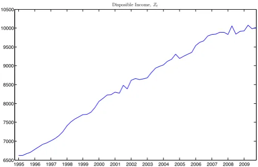
Figure 5.2 clearly shows that it is not unreasonable to assume a simple linear trending function for
a disposable income data set (a quarter data set from the first quarter of 1960 to the last quarter
of 2009 available from the Bureau of Economic Analysis at http://www.bea.gov).
The following example is the same as Example 5.2 of Li et al (2011). We use this example to
show that in some empirical models, a second–order polynomial model is more accurate than a
simple linear model.
Example 5.2. In this example, we consider the 2–year (x1t) and 30–year (x2t) Australian
1995 1996 1997 1998 1999 2000 2001 2002 2003 2004 2005 2006 2007 2008 2009 6500
7000 7500 8000 8500 9000 9500 10000 10500
[image:16.595.166.419.80.244.2]Disposible Income,Zt
Figure 5.2. Plot of the disposable income data
interest rates. Our aim is to analyze the relationship between the long–term data{x2t}and short–
term data{x1t}. We first apply the transformed versions defined byyt= log(x2t) andxt= log(x1t).
The time frame of the study is during January 1971 to December 2000, with 360 observations for
each of{yt} and{xt}.
Consider the null hypothesis defined by
H0: yt=α0+β0xt+γ0x2t+et, (5.6)
where{et} is an unobserved error process.
In case there is any departure from the second–order polynomial model, we propose using a
nonparametric kernel estimate of the form
b
g(x) =
n
X
t=1
wnt(x)
yt−αb0−βb0xt−γb0x2t
, (5.7)
where αb0 = −0.2338, βb0 = 1.4446, γb0 = −0.1374, and {wnt(x)} is as defined in (3.2), in which
K(x) = 34(1−x2)I{|x| ≤ 1} and an optimal bandwidth bhoptimal is chosen by a cross–validation
method.
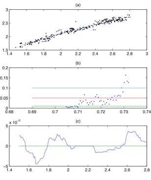
Figure 5.3 shows that the relationship betweenyt andxt may be approximately modelled by a
second–order polynomial function of the formy =−0.2338 + 1.4446x−0.1374x2.
The following example is the same as Example 4.5 of Gao, Tjøstheim and Yin (2012). We use
it here to show that a parametric version of model (4.2) is a valid alternative to a conventional
integrated time series model in this case.
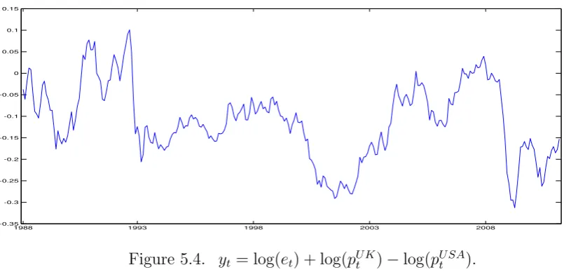
Example 5.3. We look at the logarithm of the British pound/American dollar real exchange
rate, yt, defined as log(et) + log(pU Kt ) −log(pU SAt ), where {et} is the monthly average of the
1.4 1.6 1.8 2 2.2 2.4 2.6 2.8 3 1.5
2 2.5 3
(a)
0.680 0.69 0.7 0.71 0.72 0.73 0.74
0.05 0.1 0.15 0.2
(b)
1.4 1.6 1.8 2 2.2 2.4 2.6 2.8
!5 0 5x 10
[image:17.595.140.449.79.447.2]!3 (c)
Figure 5.3: (a) provides the scatter chart of (yt, xt) and a nonparametric kernel regression plotby=mb(x); (b) givesp–values of the test for different bandwidths; and (c) is the plot ofbg(x) and its values are
between−5×10⁻³and 5×10⁻³.
data come from website: http://www.rateinflation.com/ and the exchange rate data are available
at http://www.federalreserve.gov/, spanning from January 1988 to February 2011, with sample
sizen= 278.
Our estimation method suggests that{yt}approximately follows a threshold model of the form
yt=yt−1−1.1249yt−1I[|yt−1| ≤0.0134] +et. (5.8)
Note that model (5.7) indicates that while {yt}does not necessarily follow an integrated time
series model of the formyt=yt−1+et,{yt}behaves like a “nearly integrated” time series, because
the nonlinear component g(y) =−1.1249y I[|y| ≤0.0134] is a ‘small’ departure function with an
upper bound of 0.0150.
1988 1993 1998 2003 2008 -0.35
[image:18.595.77.485.68.262.2]-0.3 -0.25 -0.2 -0.15 -0.1 -0.05 0 0.05 0.1 0.15
Figure 5.4. yt= log(et) + log(pU Kt )−log(pU SAt ).
This paper has discussed a class of “nearly linear” models in Sections 2–4. Section 2 has
summarised the history of model (1.1) and then explained why model (1.1) is important and has
different theory to what has been commonly studied for model (1.2). Sections 3 and 4 have further
explored such models to the nonstationary cases with the co-integrating case being discussed in
Section 3 and the autoregressive case being discussed in Section 4. As shown in Sections 3 and 4,
respectively, while the conventional “local–time” approach is applicable to establish the asymptotic
theory in Proposition 3.1, one may need to develop the so–called “Markov chain” approach for the
establishment of the asymptotic theory in Proposition 4.2.
As discussed in Remark 4.1, model (4.2) introduces a class of non–integrated but “nearly
integrated” autoregressive time series models. Such a class of nonstationary models, along with a
class of nonstationary threshold models proposed in Gao, Tjøstheim and Yin (2012), may provide
existing literature with two new classes of nonlinear nonstationary models as alternatives to the
class of integrated time series models already commonly and popularly studied in the literature.
It is hoped that such models proposed in (4.2) and Gao, Tjøstheim and Yin (2012) along with
the technologies developed could motivate us to develop some general classes of nonlinear and
nonstationary autoregressive time series models.
7. Acknowledgments
The author acknowledges benefits from collaborations and discussion with his co–authors in the
last few years, particularly with Jia Chen, Maxwell King, Degui Li, Peter Phillips, Dag Tjøstheim
and Jiying Yin. The author also acknowledges useful comments and suggestions by Biqing Cai
and Hua Liang. Thanks go to the Australian Research Council for its financial support under the
Discovery Grants Scheme under Grant Number: DP1096374.
Appendix A
lemmas for the proof of Proposition 4.2.
Let {yt} be a null–recurrent Markov chain. It is well–known that for a Markov chain on a
countable state space which has a point of recurrence, a sequence split by the regeneration times
becomes independent and identically distributed (i.i.d.) by the Markov property (see, for example,
Chung 1967). For a general Markov process that does not have an obvious point of recurrence, as
in Nummelin (1984), the Harris recurrence allows one to construct a split chain that decomposes
the partial sum of the Markov process {yt} into blocks of i.i.d. parts and the negligible remaining
parts.
Let zt only take the values 0 and 1, and {(yt, zt), t≥0} be the split chain. Define
τk =
inf{t≥0 : zt= 1}, k= 0,
inf{t > τk−1 : zt= 1}, k≥1,
(A.1)
and denote the total number of regenerations in the time interval [0, n] by T(n), that is,
T(n) =
max{k: τk≤n}, if τ0≤n,
0, otherwise.
(A.2)
Note that T(n) plays a central role in the proof of Proposition 4.2 below. WhileT(n) is not
observable, it may be replaced by πTs(C(In)
C) (see, for example, Lemma 3.6 of Karlsen and Tjøstheim
2001), where TC(n) = Pnt=1I[yt∈C], C is a compact set and IC is the conventional indicator
function. In addition, Lemma 3.2 of Karlsen and Tjøstheim (2001) and Theorem 2.1 of Wang
and Phillips (2009) imply thatT(n) is asymptotically equivalent to√nLB(1,0), whereLB(1,0) =
limδ→0 21δ
R1
0 I[|B(s)|< δ]dsis the local–time process of the Brownian motion B(r).
We are now ready to establish some useful lemmas before the proof of Proposition 4.2. The
proofs of Lemmas A.1 and A.2 below follow similarly from those of Lemmas 2.2 and 2.3 of Gao,
Tjøstheim and Yin (2012), respectively.
Lemma A.1 Let Assumption 4.2(i)(ii) hold. Then as n→ ∞
1 √
n
[nr]
X
t=1
et+
1 √
n
[nr]
X
t=1
g(yt−1)=⇒D σe B(r) +M1 2(
r) µg ≡Q(r), (A.3)
where M1
2(r), µg and Q(r) are the same as defined in Proposition 4.2.
Lemma A.2 Let Assumption 4.2 hold. Then as n→ ∞
1
T(n)
n
X
t=1
yt−1g(yt−1) →P
Z ∞
−∞
yg(y)πs(dy), (A.4)
1
n2
n
X
t=1
yt2−1 →D
Z 1
0
Q2(r) dr, (A.5)
1
n
n
X
t=1
yt−1et →D
1 2
Proof of Proposition 4.2. The proof of the first part of Proposition 4.2 follows from Lemma A.2 and
nβb−1= 1
n2
n
X
t=1
yt2−1
!−1
1
n
n
X
t=1
yt−1et
!
+ 1
n2
n
X
t=1
yt2−1
!−1
T(n)
n
1
T(n)
n
X
t=1
yt−1g(yt−1)
!
. (A.7)
The proof of the second part of Proposition 4.2 follows similarly from that of Proposition
3.1(ii).
References
Chen, J., Gao, J. and Li, D. (2011). Estimation in semiparametric time series models (invited paper).
Statistics and Its Interface4, 243–252.
Chen, J., Gao, J. and Li, D. (2012). Estimation in semiparametric regression with nonstationary regressors (http://www.bernoulli-society.org/index.php/publications/bernoulli-journal/bernoulli-journal-papers). Forthcoming inBernoulli18.
Chung, K. L. (1967). Markov Chains with Stationary Transition Probabilities. Springer–Verlag, 2nd Edition.
Fan, J. and Gijbels, I. (1996). Local Polynomial Modeling and Its Applications. Chapman & Hall, London.
Fan, J., Wu, Y. and Feng, Y. (2009). Local quasi–likelihood with a parametric guide. Annals of Statistics 37, 4153–4183.
Fan, J. and Yao, Q. (2003). Nonlinear Time Series: parametric and nonparametric methods. Springer, New York.
Gao, J. (1992) Large Sample Theory in Semiparametric Regression. Doctoral Thesis at the Graduate School of the University of Science and Technology of China, Hefei, China.
Gao, J. (1995). Parametric test in a partially linear model. Acta Mathematica Scientia(English Edition)
15, 1–10.
Gao, J. (2007). Nonlinear Time Series: semi– and non–parametric methods. Chapman & Hall, London.
Gao, J. and Gijbels, I. (2008). Bandwidth selection in nonparametric kernel testing. Journal of the American Statistical Association484, 1584-1594.
Gao, J., King, M. L., Lu, D. and Tjøstheim, D. (2009a). Nonparametric specification testing for nonlinear time series with nonstationarity. Econometric Theory25, 1869–1892.
Gao, J., King, M. L., Lu, D. and Tjøstheim, D. (2009b). Specification testing in nonlinear and nonsta-tionary time series autoregression. Annals of Statistics37, 3893–3928.
Gao, J., Tjøstheim, D. and Yin, J. (2012). Estimation in threshold autoregressive models with a stationary and a unit root regime (http://www.buseco.monash.edu.au/ebs/pubs/wpapers/2011/wp21-11.pdf). Forthcoming inJournal of Econometrics170.
Glad, I. (1998). Parametrically guided nonparametric regression. Scandinavian Journal of Statistics25, 649–668.
Granger, C. W. J., Inoue, T. and Morin, N. (1997). Nonlinear stochastic trends. Journal of Econometrics 81, 65–92.
H¨ardle, W., Liang, H. and Gao, J. (2000). Partially Linear Models. Springer Series in Economics and Statistics. Physica–Verlag, New York.
Juhl, T. and Xiao, Z. (2005). Partially linear models with unit roots. Econometric Theory21, 877–906.
Karlsen, H. A. and Tjøstheim, D. (2001). Nonparametric estimation in null recurrent time series. Annals of Statistics29, 372–416.
Li, D., Gao, J., Chen, J. and Lin, Z. (2011). Nonparametric estimation and specification testing in nonlinear and nonstationary time series models. Working paper available at www.jitigao.com.
Li, Q. and Racine, J. (2007). Nonparametric Econometrics: theory and practice. Princeton University Press, Princeton.
Martins–Filho, C., Mishra, S. and Ullah, A. (2008). A class of improved parametrically guided nonpara-metric regression estimators. Econometric Reviews27, 542–573.
Masry, E. and Tjøstheim, D. (1995). Nonparametric estimation and identification of nonlinear ARCH time series. Econometric Theory11, 258–289.
Nummelin, E. (1984). General Irreducible Markov Chains and Non-negative Operators. Cambridge Uni-versity Press.
Owen, A. (1991). Empirical likelihood for linear models. Annals of Statistics 19, 1725–1747.
Park, J. Y. and Phillips, P. C. B. (2001). Nonlinear regressions with integrated time series. Econometrica 69, 117–162.
Robinson, P. M. (1988). Root–N–consistent semiparametric regression. Econometrica56, 931–964.
Ter¨asvirta, T., Tjøstheim, D., Granger, C. W. J. (2010). Modelling Nonlinear Economic Time Series. Oxford University Press, Oxford.
Tong, H. (1990). Nonlinear Time Series: a Dynamical System Approach. Oxford University Press, Oxford.
Wang, Q. Y. and Phillips, P. C. B. (2009). Asymptotic theory for local time density estimation and nonparametric cointegrating regression. Econometric Theory25, 710-738.
Wang, Q. Y. and Phillips, P. C. B. (2011). Asymptotic theory for zero energy functionals with nonpara-metric regression application. Econometric Theory27, 235–259.
Wang, Q. Y. and Phillips, P. C. B. (2012). Specification testing for nonlinear cointegrating regression. Forthcoming inAnnals of Statistics40.