Valuating New Product Development Project with a Stochastic Volatility Model

http://www.scirp.org/journal/jmf ISSN Online: 2162-2442

ISSN Print: 2162-2434

Valuating New Product Development Project with

a Stochastic Volatility Model

Chengru Hu

1

, Chulhee Jun

2

, Maggie Foley

3

1_{State University of New York at Canton, Canton, NY, USA} 2_{University of Macao, Macao, China}

3_{Jacksonville University, Jacksonville, FL, USA}

Abstract

In this study, we develop an option-based model to valuate New Product Develop-ment (NPD) projects in which manageDevelop-ment has the flexibility to abandon the project upon completion if the value of the established product falls below the required in-vestment outlay. In the analysis, we explicitly consider the fact that the level of prod-uct volatility changes across development stages, as well as the stochastic nature of competition erosion. A closed-form solution is derived under a simplifying assump-tion of independence between product volatility and other stochastic processes con-sidered in the model. The complete model is solved numerically by using Monte Carlo simulation. Our result indicates that ignoring the stochastic natures of product development uncertainty and competition erosion introduces a severe undervalua-tion bias. Such a bias worsens when 1) current product value is close to the required investment cost (so that the NPD project is nearly “at-the-money”); 2) development duration lengthens; 3) competition is intense; 4) the window of profitable opportu-nity lengthens, and 5) the market and the developing firm are more risk-prone (less risk-averse).

Keywords

Real Option, Strategic Flexibility, New Product Development, Stochastic Volatility

1. Introduction

New Product Development (NPD) is fundamental to stimulating economic growth for business organizations. Successful NPDs not only support important business activities that over time contribute to long-run business profitability, but also provide firms with sufficient cutting edges in competitive battles.

How to cite this paper: Hu, C.R., Jun, C. and Foley, M. (2016) Valuating New Product Development Project with a Stochastic Vola-tility Model. Journal of Mathematical Fi- nance, 6, 975-1001.

http://dx.doi.org/10.4236/jmf.2016.65064 Received: September 19, 2016

Accepted: November 26, 2016 Published: November 30, 2016

Copyright © 2016 by authors and Scientific Research Publishing Inc. This work is licensed under the Creative Commons Attribution International License (CC BY 4.0).

Recognition of the importance of NPD to business prosperity has triggered consi-derable research interests from a variety of domains including marketing, strategic management and economics. Of all widely studied research topics, none is more chal-lenging and has received more attention than the valuation of NPD investments. When corporate resources are limited, competition is intense, and the cost associated with NPD investment is significant; therefore, the accuracy with which NPD investments can be evaluated becomes critically important.

Traditionally, the Net Present Value (NPV) rule is recommended for analyzing in-vestment decisions. The NPV rule helps decision makers choose between two alterna-tives: accepting or rejecting an investment opportunity. However, it is widely accepted that the majority of the investments firms make are dynamic in that decision makers do more than just accept or reject an investment opportunity using information available at the time of the decision. Upon arrival of additional information, decision makers update their beliefs about the profitability of the investment and may choose to defer, expand, contract, or shut down temporarily and later restart the investment project (Trigeorgis and Mason [1]; Trigeorgis [2]; among others). Flexibility to revise actions based on future events enables management to amplify future gain or mitigate loss in face of favorable or unfavorable events, and thus carries real value. Standard NPV anal-ysis places investment analanal-ysis into a static framework and totally ignores the value of strategic flexibilities; consequently it will result in an undervaluation of investment pro- jects (Myers [3]; Kester [4]; Amram and Kulatilaka [5]; etc).

Alternatively, academic researchers adopt the principles of option pricing in analyz-ing investment decisions. Strategic flexibilities that allow decision makers to alter the course of investment at later dates resemble options written upon the underlying assets (Caballero [6]; Kulatilaka [7]; Baldwin and Clark [8] and [9]; etc). Therefore the op-tion-based approach, or the real option approach, provides more appropriate represen-tations of investment dynamics and will effectively mitigate the documented underval-uation problems.

In this study, we develop an option-based model to evaluate a NPD project that al-lows management to abandon the project upon completion. NPD is a risky process. Previous studies document high product failure rates and significant costs to sponsor-ing company upon product failure (Booz-Allen and Hamilton [10]; Mansfield [11]; Panne, Beers, and Kleinknecht [12]). Flexibility to abandon the project given unfavora-ble outcomes effectively reduces downside loss, and is a valuaunfavora-ble strategic tool. Ignoring it would lead to a significant undervaluation problem.

Se-condly, we explicitly consider the stochastic nature of industrial competition on NPD valuation. Industrial competition erodes the value of NPD projects, long before the es-tablishment of a product. Previous studies on the impact of competition erosion as-sume the rate of erosion to be either constant or take a deterministic functional form. We recognize that competition erosion depends on stochastic competitor arrivals and uncertainty about the future investment environment. Consequently, we allow the rate of competition erosion to be random in our NPD valuation model.

The dynamics underneath our stochastic (product) volatility with stochastic compe-tition model (SVSCM) is very general in which previously studied project dynamics are special cases of ours. For example, by assuming a constant level of product volatility, our model reduces to a stochastic competition with Constant (product) Volatility Mod-el (CVM). By further restricting that change in the rate of competition erosion to zero, our model is further reduced to the Constant Competition with constant product vola-tility Model (CCM).

We derive a closed-form solution to SVSCM under a simplifying assumption that a change in product volatility is independent of changes in new product value and com-petition erosion. We further provide a numerical solution to the full-scale SVSCM us-ing Monte Carlo simulations. We design a control variate methodology to obtain accu-rate (as measured by standard deviation of simulation results) estimations of project value with low computation cost (as measured by the number of simulation repetitions). We then examine the valuation benefit of admitting the stochastic nature of develop-ment uncertainty and industrial competition based on simulation results. Our results suggest valuation under SVSCM is much higher than those under CVM and CCM un-der various scenarios. We find that the unun-dervaluation bias in CVM and CCM becomes severe when 1) current product value is close to required investment cost (so that the NPD project is nearly “at-the-money”); 2) development duration lengthens; 3) compe-tition is intense; 4) the window of profitable opportunities lengthens, and 5) markets and developing firms are more risk-averse.

The major contribution of this study is that it highlights the importance of additional volatility from changing project uncertainty and competition erosion in the valuation of NPD projects. Previous studies assume constant product uncertainty and/or constant competition erosion. We argue that these assumptions are inadequate to capture the dynamic nature of NPD development. Real option theory suggests that under dynamic management the value of an NPD project increases with the uncertainty. Changing competition erosion and product volatility adds to a project’s uncertainty, which in-creases the likelihoods of both significant gain and loss. The option to abandon effec-tively limits downside losses, but allows a developing firm to reap potential gains; con-sequently additional uncertainty implies higher valuation. Our results indicate that ig-noring the stochastic nature of competition erosion, and especially changing level product volatility will introduce severe undervaluation bias, and lead to an underin-vestment problem.

Section 3 describes the dynamics of the NPD project, derives a valuation model, and provides a solution to under risk-neutral representation. In Section 4, a closed-form solution is provided assuming independence between change in product volatility and other stochastic variables. Section 5 utilizes a Monte Carlo simulation technique to numerically solve the value of the NPD project. We also examine the marginal contri-bution of our derived model under various scenarios. We then conclude our study in Section 6.

2. Literature Review

The conventional (static) DCF technique assumes that an investment, once started, will be operated continuously until the end of its expected useful life. The valuation crite-rion is based on present values of expected outputs/inputs discounted at a risk-adjusted rate, i.e.

(

)

0 NPV

1

T

t t t t

adj

E CF I

r

=

 − 

 

=

+

∑

 (1)

where CF t is period t cash flow from the investment; radj is a discount rate adjusted

for risk associated with the investment; T is expected useful life of the investment (it is the required investment outlay required at time t); and E[·] is the expectation operator. Investments with positive (negative) NPVs increase (decrease) the wealth of a firm’s owners; therefore should be accepted (rejected).

Since seminal work by Myers [3], the option-pricing framework has been applied to value investment decisions and contractual claims on corporate assets. Managerial flexibilities to alter the investment course at later stages resemble options written upon the underlying real assets (Myers [3]; Kester [4]). Table 1 suggests that there exist striking similarities between “options” on real assets (thereafter, real options) and fi-nancial options. As a result, it has been suggested that fifi-nancial option-pricing theories could be utilized to measure values of managerial flexibilities.

The problems with static NPV easily can be solved with a real option approach. First of all, the real option approach relies on contingent claim analysis, and replicates future cash flows from a potential investment using those of a portfolio of existing assets. This “cash flow equivalent” portfolio has the same payoff as the investment under consider-ation. In the absence of arbitrage opportunities, the value of investment is the value of this replicating portfolio. All individuals, regardless of their subjective estimates of fu-ture cash flow distributions, agree on the valuation. Secondly, as fufu-ture cash flow esti-mates are independent of individual risk preference, risk-neutral probabilities and a risk-free rate are used in the valuation. Finally, operating flexibilities are models as a set of boundary conditions, so that initial investment strategies (and investment outcomes) can be altered upon realization of future events.

So far, the real option approach has been adopted in the valuation of various types of managerial flexibilities. Examples include (but not limited to) 1) option to defer (Pad-dock, Siegel and Smith [19]; McDonald and Siegel [20] [21]; etc.); 2) time to build (Majd and Pindyck [22]; Trigeorgis [23]; etc.); 3) option to expand (contract) (Brennan and Schwartz [24]; McDonald and Siegel [21]; etc.); 4) option to switch (Kensinger [25]); and 5) option to abandon (Myersand Majd [26]); etc.

[image:5.595.195.547.584.705.2]

Option to abandon a project at a later stage is an important strategic tool especially when project development faces high level of uncertainty and severe competition, for example a NPD project. A NPD project typically involves technology whose future is virtually unknown. As evidenced by unexceptionally high failure rates among NPD projects (Mansfield et al. [11]; Booz, Allen and Hamilton [10]; etc.), product construc-tions are usually unstable with low confidence in the product’s success. Industry com-petition erodes the value of a NPD project long before the establishment of a product, as potential consumers waiting for the new product are diverted to competing products Table 1. Comparison of financial and real options.

Financial Options Real Options

- Current stock price - Current value of asset

- Stock return volatility - Variance of rate of change in asset value - Exercise price - (Per unit) development cost

of similar technologies, reducing the potential market for the new product. The ability to abandon the project when product value at a future time (e.g. upon completion) falls below required thresholds would effectively curb downside loss but enable firms to reap upside potential gain if the product turns out to be a success; consequently, the ability to abandon represents real value. Intuitively, the value of this strategic tool increases with uncertainty.

Chen, Ho, Ik and Lee [27] are among the first to adopt real option approach into NPD evaluation. Chen et al consider the flexibility to abandon in the valuation of a NPD project. They take into consideration the effect of industrial competition on the value of the new product. Schwartz [28] uses real option approach to value patents and patent- protected R & D projects in pharmaceutical industry. His model implicitly con-siders uncertainty in cost-to-completion, uncertainty in cash flows to be generated, and possibility of catastrophic events. In both studies, volatility of innovative project are assumed to be constant during development period. However, there exists abundant evidence, from both marketing and economic literature, that suggest risk levels asso-ciated with NPDs vary as product development progresses (Contractor and Narayanan [16]; Fahey and Narayanna [15]; Nelson and Winter [14]; Sahal [13]; etc.). A typical NPD involves seeding, startup, breakthrough, and new product commercialization phases. A firm’s focus changes across development stages. The early stage involves idea testing with a major source of uncertainty being the feasibility of the innovation con-cept. In later phases (e.g. start-up, breakthrough), a firm focuses on materializing the concept. Consequently, most uncertainties come from finding technical solutions. Fi-nally, during product commercialization, the firm’s major concern shifts to competi-tions and especially the demands of the market. Cash flows resulting from the new product are less dependent on the firm’s technological capability. As uncertainty levels across phases vary with shifting development focuses, assuming constant product vola-tility in project valuation is apparently inappropriate. Such assumption will under-es- timate NPD uncertainty and under-value both the strategic ability to abandon NPD projects.

3. New Product Development Valuation Model

In this section, we propose an option-based valuation model to capture the value of flexibility to abandon NPD projects at later stage. We explicitly consider the impacts of varying project volatility and stochastic competition on values of NPD projects.

Suppose the firm under consideration is developing a new product. The development will last T months. Upon product completion, if value of the established product falls below required production costs K, the firm will choose to abandon the project. The value of NPD project at time t, B S t

(

( ) ( ) ( )

,σ t ,δ t ,t

)

, is a function of the value of

product under development, S t

( )

, and the loss in value (from sales reduction) due to

competition δ

( )

t .

3.1. Product Value

Geometric Brownian motion with the following form:

( )

( ) ( )

( ) ( )

dS t =_µ δ− t _S t dt+σ_S t S t dω_S (2) where μ is the expected value appreciation for the product; δ

( )

t is time t rate of

competition erosion; δS

( )

t is time t instantaneous product volatility; and dωS is the

increment of a standard Wiener process with E

(

dω_S

)

=0, and var d

(

ω_S

)

=dt

3.2. Product Volatility

We model instantaneous product volatility, σS

( )

t , with a stochastic process to capture

the fact that the level of uncertainty changes as the NPD project progresses. Firms tend to develop products in their existing business line; consequently, product volatility normally reverts to the risk of firm’s existing assets in the long-run (Chung and Cha-roenwong [29]; Miles [30]). We therefore use the following process to model instanta-neous product volatility σS

( )

t :

( )

( )

dσ_S t =kσ β σ− _S t dt+σ ωσd σ (3)

where k_σ is the speed of the adjustment; β is the long-term reversion level; σ_σ is the instantaneous volatility; and dω_σ is the increment of a standard Wiener process with

(

d

)

0

E ωσ = and var d

(

ωσ

)

=dt. We further assume instantaneous product volatility

is correlated with product value movements (i.e. cov d

(

ω_S, dω_σ

)

=ρ_Sσdt>0) but is in-dependent with competition erosion change (therefore cov d

(

ωδ, dωσ

)

=0).

3.3. Competition Erosion

Loss in value due to competition represents value outflows that will not accrue to the developing firm. This resembles dividend-like convenience yield on real assets (Fama and French [31][32]; Gibson and Schwartz [33]). In the long-run, competition tends to move back towards an equilibrium level due to factors such as marginal production costs (Gibson and Schwartz [33]; Demers [34]; Bjerksund and Ekern [35]). Conse-quently, we model rate of erosion due to industrial competition, δ

( )

t , with the

fol-lowing mean-reverting process, i.e.

( )

( )

dδ t =k_{δ }α δ− t _dt+σ ω_δd _δ (4) where kδ is the speed of reversion; α represents the equilibrium long-run average

( )

t

δ reverts to; σδ is the instantaneous volatility; and dωδ is the increment of a

standard Wiener motion with E

(

dω_δ

)

=0 and var d

(

ω_δ

)

=dt.

It is assumed competition erosion is positively correlated with product value, i.e.

(

)

cov dω_S, dω_δ =ρ_Sδdt>0, where ρ_Sδ is the correlation coefficient. Intuitively, when the value of an innovative product is high (low), competitors enter (exit) the market. The supply of products with similar features increases (decreases), putting downward (upward) pressure on the market share the new product could obtain.

3.4. Boundary Condition

product falls below the required investment outlay, K, upon product complete at time T. Project value upon considering this flexibility can be modeled as:

( )

, _S

( ) ( )

, , max

( )

, 0

B S T_ σ T δ T T_= _S T −K _ (5)

where S T

( )

is time T product value; and K is the requirement value threshold to

ac-cept the product.

Risk neutral representation of NPD dynamics (2), (3) and (4) could be established by adjusting the actual movements of underlying state variables with corresponding risk premiums (Cox, Ingersoll and Ross [36]). Value movements governed by stochastic processes (2), (3) and (4), the corresponding risk neutralized processes are given as:

( )

( ) ( )

( ) ( )

ˆ ˆ ˆ _ˆ ˆ

dS t =_r−

δ

t _S t dt+

σ

_S t S t d

ω

_S (2)*

( )

{

( )

}

ˆ ˆ

dσS t = kσ β σ− S t −λ σσ σ dt+σ ωσd σ (3)*

( )

{

( )

}

ˆ ˆ

d

δ

t = k_{δ }

α δ

− t _−

λ σ

_{δ δ} dt+

σ ω

_δd _δ (4)* where r is the risk free rate; λδ and λσ are the market prices of risk for competition

erosion and stochastic volatility, respectively. λδand λσ are assumed to be constant.

With Ito’s Lemma, it can be shown that in the absence of arbitrage opportunities NPD value following the risk-adjusted processes (2)*, (3)* and (4)* must satisfy the fol-lowing partial differential equation (for simplicity, we drop the “^” from the notation):

(

)

(

)

(

)

2 2 2 2

1 1 1

2 2 2

0

SS S S S S S S S S

S t

B S B B B S B S B S r

B k B k B rB

δδ δ σσ σ δ δ δ σ σ σ

δ δ δ δ σ σ σ σ

σ σ σ ρ σ σ ρ σ σ δ

α δ λ σ β σ λ σ

+ + + + + −

 

+ _ − − _+ _ − − _− − = (6)

subject to boundary condition (5).

Equation (6) doesn’t depend on investor risk preference. Therefore, its solution has a risk-neutral representation (Cox and Ross [37]). For simplicity, we evaluate NPD value at time t = 0. The value of NPD project at time 0 is:

( ) ( )

0 , 0 ,

( )

0 , 0 e ˆ0 max

(

, 0

)

rT

S T

B S_ δ σ _= − E _ S −K _ (7)

where _Eˆ

( )

_{⋅ is the risk-adjusted expectation operator.}

NPD value at evaluation can be calculated by determining the time T distribution

(

_T , , , , , ,

)

p S k_σ k r_δ α β σ σ_{σ δ}

and (7) can be transformed into:

( )

( ) ( )

(

0 , 0 , 0 , 0

)

e

(

)

(

, , , , , ,

)

d

T

rT

S _{S K} T T T

4. Closed-Form Solution under Simplifying Assumption

With movement of project value governed by processes specified in Section 3, there ex-ists no closed-form solution to Equation (8). However, under the simplifying solution that volatility change is independent of NPD change (therefore cov d

(

ω_S, dωσ

)

=0)1, a closed-form solution to Equation (8) can be achieved. Our derivation proceeds in two steps. First we show that, given that change in product uncertainty is independent of both product value movement and competition erosion, NPD value under each sto-chastic volatility path follows a log-normal distribution. Next, we extend the results of Stein and Stein [38] to derive the close-form solution to NPD value at time 0.

Define Θ as the point in the probability space that labels the stochastic path. For each

path Θ, we define

( )

1 2 2 , 0 1 d T T S T

σΘ σ τ τ

 

=  



∫

 as mean volatility of the given sample path

2_.

Under the assumptions that NPD volatility is independent of both NPD value change and industrial competition defined in (2)* and (4)*, (8) can be expressed as3_:

(

)

(

)

(

,

)

(

,

)

0

, ,

e , , , , , , d d

T

S

rT

T T T T T

S K

B S

S K g S k_σ k r_{δ δ} S m _σ

δ σ

α β σ σ σ σ σ

∞ ∞

−

Θ Θ Θ

=

 

=  − 

 

 

∫

∫

(9)

where g S

( )

T ⋅ is the time T probability density function of ST condition on given

volatility path (consequently mean volatility

σ

Θ,T) and parameters kσ,k rδ, , , ,α β σδ.

(

,T

)

m

σ

Θ

σ

_σ is the probability density function of σΘ under assumption of risk neu-

trality, where

{

,

}

(

,

)

d ,

b

T T T

a

prob_Θ b>σ_Θ >a =

∫

m σ_Θ σ_σ σ_Θ . To simply the notation, we

will use m

( )

σ_Θ

for m

(

σ

Θ,T

σ

σ

)

.

The inner integral in (9) represents NPD value under a path Θ. It represents solution to the following partial differential equation (Cox, Ingersoll and Ross [36], Theorem 3):

(

)

(

)

2 2 2

, ,

1 1

2 2

0

SS T S S T S

t

B S B B S B S r

B k B rB

δδ δ δ δ δ

δ δ δ δ

σ σ ρ σ σ δ

α δ λ σ

Θ + + Θ + −

+ _ − − _ − = (10)

with boundary condition B S T_

( ) ( )

,δ T ,T_=max_S T

( )

−K, 0_.

Appendix A shows that with a selected sample path, the resulting distribution of new product’s value at time T is log-normal distributed, with a density function given by:

(

)

(

)

(

)

2 2 0 , 2 log 0.5* 1 , exp 2 2π T F T T F F T

S S r T

L S T S T σ σ σ σ Θ  _{ − − }      = _− _    

in which 2 2

( )

2

( )

, 2 ,

F T δA T T δ SδA T

σ = σ_Θ +σ − σ σ ρ_{Θ and} A T

( )

1 e k Tδ k δ

−

 

= −_{  .}

1_{That is, 0.}

Sσ

ρ = With this assumption, the instantaneous product volatility is independent of both NPD value movements and industry competition effect.

2_Note

,T

σΘ is a random variable.

Given that the NPD value at time T under each sample path of σS follows

lognor-mal distribution, the exact distribution of NPD value at time T can be expressed as an average of lognormal distributions, averaged via the distribution function of σ_Θ:

(

T , , , , , ,

)

(

T,

) ( )

T d

p S kσ kδ rα β σ σσ δ =

∫

L S σΘ m σΘ σ_Θ (11)

In Appendix B, we show that NPD value distribution (11) is given by:

(

)

( )

(

)

(

2

)

( )

(

)

( )

0

2 0.25 *

1 1.5 2.5 log

, , , , , ,

0.25

2π e e e d

2

T

T

B T i S S rT

rT T

p S k k r

T

S I

σ δ σ δ

η _η

η

α β σ σ

η η ∞ − + − − − − =−∞  +    =    

∫

(12)

where

( )

2

( )

(

2

)

1 S 2

B T =_

σ

_δA T −

ρ

_δ T_ .

With time T product value distribution p S k

(

_{T σ},k r_δ, , , ,α β σ σ_σ, _δ

)

, NPD value at current time could be calculated as:

(

)

(

) ( )

(

2

)

( ) ( )

0

0.25 *

1 1.5 2.5 2 log

, , e

1

2π e e e d d

4 2

T T

rT S

B T _{i S S rT}

rT

T T T

S K

B S

T

S K S η I η S

η

δ σ

η

η

− ∞ − − − ∞ − + − = =−∞ =      × − _{ } + _{  }      

∫

∫

(13)

5. Numerical Solution

Even under the simplifying assumption, the closed-form solution given in (13) requires integration with imaginary functions; therefore the calculations are very complex and time-consuming. To solve for NPD value under the full model (8), we implement a Monte Carlo simulation to numerically find its solution. There are two major concerns to any Monte Carlo simulation, namely accuracy (as measured by standard deviation of estimates) and computational cost (as measured by number of simulation repetitions). In order to improve the accuracy of Monte Carlo estimates while reducing the number of simulation repetitions performed, a control variate methodology is adopted. The ba-sic idea is to replace the integration Equation (8) with one that has an analytic solution, under the assumption that product volatility, σS

( )

t , is deterministic. Monto Carlo

simulation is used to simulate the difference between the Equation (8) and the fied solution. A detailed explanation of the control variate methodology and the simpli-fied solution utilized are introduced in the Appendix.

5.1. Base Case Result

[image:11.595.195.554.90.272.2]

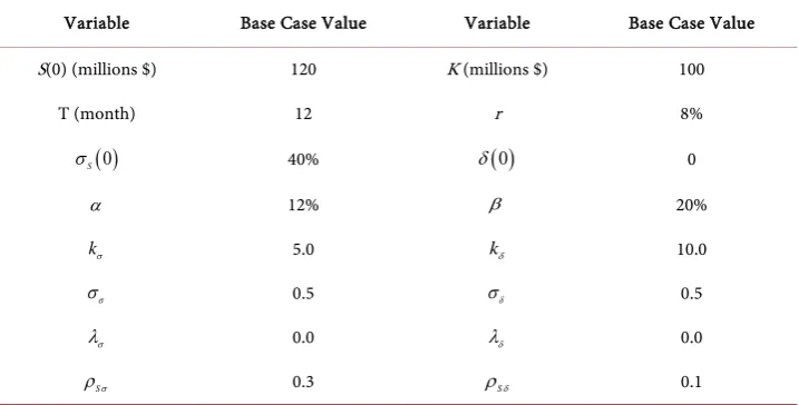
Table 2. Summary of base case simulation parameters.

Variable Base Case Value Variable Base Case Value

S(0) (millions $) 120 K (millions $) 100

T (month) 12 r 8%

( )

0

S

σ _40% δ

_{( )}

0 0

α _12% β _20%

kσ 5.0 kδ 10.0

σ

σ 0.5 σδ 0.5

σ

λ 0.0 λδ 0.0

Sσ

ρ _0.3 ρ_Sδ 0.1

Parameter values are based on the simulations by Chen et al. (2001) and Schwartz (2004).

and its long-term level, α, is set to be 12%. Initially, the product volatility, σ_S

( )

0 , is 40%, and its long-term equilibrium level, β, is 20%. σσ _and σδ are set to be 0.5 and

0.5, respectively. The values of reversion rates k_σ and k_σ are set at 10.0 and 5.0. Fi-nally, the correlation coefficient between dωS and dωσ, ρSσ, is 0.3, while the

corre-lation coefficient between dω_δ and dωS, ρSσ, is 0.1. Table 2 summarizes the base

case values and the value ranges for variables used in the new product valuation model. Table 3 reports simulated NPD values with the control variate methodology intro-duced in the Appendix C with 1000 replications. Increasing the number of replications by a factor of 100 reduces the standard deviation of the estimates by a factor of 10 (i.e. 1001/2_{); consequently 1000 replications offer an accurate result at reasonable}

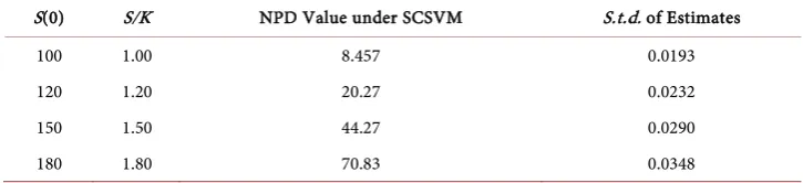
computa-tion cost. Panel A indicates that when the development duracomputa-tion increases from 3 months to 24 months (S(0) = $120 million), standard deviations for simulated NPD values increase from 0.0162 to 0.0372. Consistent with previous studies (Boyle [39]), we observe in Panel B that standard deviations of estimates increase (from 0.0193 to 0.0348) with current product value (from $120 million to $180 million, or S(0)/K ratio from 1.2 to 1.8). In summary, our simulation provides more reliable results at 1) shorter project duration and 2) lower S(0)/K ratio.

In Panel A, we observe that NPD value decreases as development duration lengthens. Intuitively, the longer it takes to establish the final product, the more potential custom-ers will be diverted to products of competitors. Our result suggests being able to bring out products faster will provide companies with significant competitive advantage over competitors.

[image:12.595.194.554.116.267.2]

Table 3. NPD base case value estimates: 1,000 replications.

Panel A: NPD value with development duration ranges between 3 months to 24 months; S(0) = $120 million. All values are in millions.

T NPD Value under SCSVM S.t.d. of Estimates

3 20.97 0.0162

6 20.85 0.0183

9 20.56 0.0215

12 20.27 0.0232

15 20.02 0.0289

18 19.79 0.0319

21 19.59 0.0337

24 19.41 0.0372

Panel B: NPD value with current product value ranges between $100 million to $180 million; T = 12 months. All values are in millions.

S(0) S/K NPD Value under SCSVM S.t.d. of Estimates

100 1.00 8.457 0.0193

120 1.20 20.27 0.0232

150 1.50 44.27 0.0290

180 1.80 70.83 0.0348

5.2. Model Comparison

In CCM, we set competition erosion (δ) and product volatility (σS) at their long-term

equilibrium levels, α = 12% and β = 20%, respectively. In CVM, competition erosion (δ) is stochastic but product volatility (σS) is constant and is set to its long-term

equili-brium level β = 20%. In SCSVM, both (δ) and product volatility (σS) are stochastic.

Table 4 provides a summary of the assumptions adopted by those models.

5.2.1. Current Product Value, S(0)

In Table 5, we change the current value of a new product within a range between $80 and $160 million, while keeping other parameters at their base case values. Given the cost of investment remains at $100 million, Table 4 provides the values of a full list of “out-of-the-month” (OTM), “at-the-money” (ATM) and “in-the-money” (ITM) pro- jects.

[image:12.595.191.554.299.382.2]

[image:13.595.195.555.114.222.2]

Table 4. Models comparison. This table lists differences in assumptions under CCM (Constant Competition Model), CVM (Constant Volatility Model), and SCSVM (Stochastic Competition with Stochastic Volatility Model).

CCM CVM SCSVM

Assumptions

1. Competition erosion is constant 2. NPD volatility is

constant

1. Competition erosion is stochastic 2. NPD volatility is

constant

1. Competition erosion is stochastic 2. NPD volatility is

stochastic Governing

stochastic process

1. S(t) follows (2) 2. σS is constant 3. δ is constant

1. S(t) follows (2) 2. σS is constant 3. δ(t) follows (4)

1. S(t) follows (2) 2. σS(t) follows (3) 3. δ(t) follows (4)

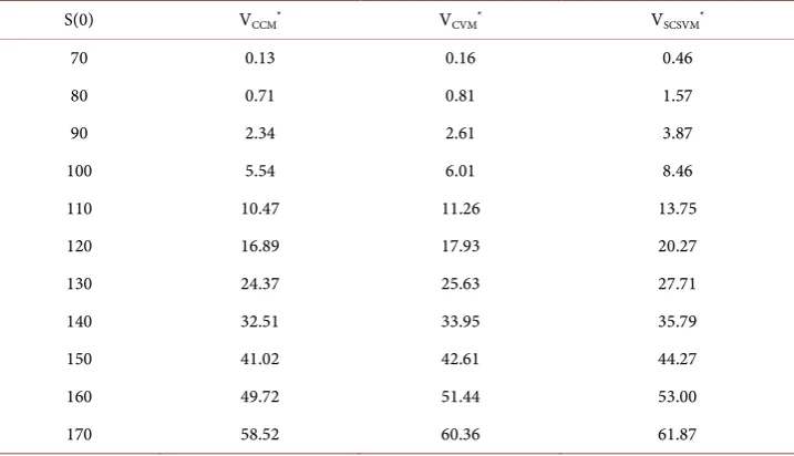
Table 5. Impact of current product value, S(0). This table reports NPD values under CCM, CVM and SCSVM models, given different initial product values, S(0). Simulation uses 1,000 replica-tions. Parameters are defined as in Table 2. All values are in millions.

S(0) VCCM* VCVM* VSCSVM*

70 0.13 0.16 0.46

80 0.71 0.81 1.57

90 2.34 2.61 3.87

100 5.54 6.01 8.46

110 10.47 11.26 13.75

120 16.89 17.93 20.27

130 24.37 25.63 27.71

140 32.51 33.95 35.79

150 41.02 42.61 44.27

160 49.72 51.44 53.00

170 58.52 60.36 61.87

*_V

SCSVM, VCCM, VCVM are NPD values derived under SCSVM, CCM and CVM, respectively.

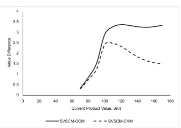
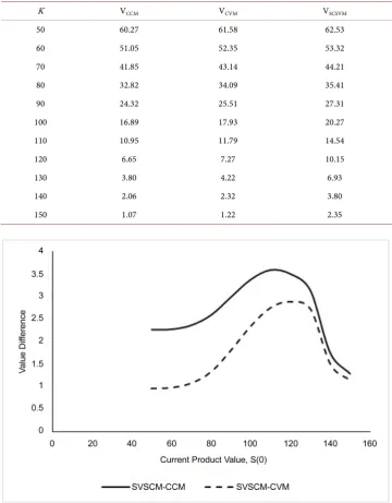
[image:13.595.194.553.280.486.2]

[image:14.595.195.554.59.312.2]

Figure 1. This figure plots the differences in values under 1) SVSCM and CVM and 2) SVSCM and CCM against initial product value, S(0). Value differences are based on simulation results reported in Table 5. All values are in millions.

protects firms from downside loss when product volatility increases; therefore, it carries more value. In the meantime, increasing volatility is more likely to result in an increase in project value. Consequently, the difference between values derived from SCSVM and CVM/CCM will widen, and will peak when project is at the money (ATM) (i.e. S(0) is nearly equal to K).

5.2.2. Investment Outlay, K

Increasing the required investment outlay K reduces project value. In Table 6, project values derived from all models decrease when development cost K rises from $60 mil-lion to $150 milmil-lion. Values of NPD projects under the CCM are the lowest and those derived from SCSVM are highest.

Figure 2 exhibits a similar pattern with Figure 1. At low (high) development cost K, a NPD project is deeply in the money (out of the money). High (low) probability of ac-cepting the project implies low (high) strategic value of abandonment. In the meantime, it is more likely that product value becomes lower (higher) at higher uncertainty. Con-sequently value difference between SCSVM and CVM/CCM shrinks (widens).

5.2.3. Development Duration, T

[image:15.595.192.553.113.575.2]

Table 6. Impact of investment outlay, K. This table reports NPD values under CCM, CVM and SCSVM models, given different product development cost, K. Simulation uses 1,000 replications. Parameters are defined as in Table 2. All values are in millions.

K VCCM VCVM VSCSVM

50 60.27 61.58 62.53

60 51.05 52.35 53.32

70 41.85 43.14 44.21

80 32.82 34.09 35.41

90 24.32 25.51 27.31

100 16.89 17.93 20.27

110 10.95 11.79 14.54

120 6.65 7.27 10.15

130 3.80 4.22 6.93

140 2.06 2.32 3.80

[image:15.595.193.553.113.574.2]

150 1.07 1.22 2.35

Figure 2. This figure plots the differences in values under 1) SVSCM and CVM and 2) SVSCM and CCM against development cost, K. Value differences are based on simulation results re-ported in Table 6. All values are in millions.

will result in higher competition erosion and lower the product value. We name this the “competition erosion effect” of T.

We at first vary only the development duration T within 3 to 24 months, but leave all other parameters at their base case values. Table 7 indicates that, in this scenario, “competition erosion effect” dominates the “value increase effect” - NPD values gener-ated by all three models decrease uniformly when development duration T lengthens. This highlights the importance of speeding up the product development process. It has been documented that Japanese companies shorten the product development process by overlapping investment phases(Takeuchi and Nonaka [41]); that firms accommo-date rapid product introductions by increasing spending to product development (Stalk [42]); and that firms implement multi-task processing and operations implification to accelerate the product development process (Millson, Raj and Wilemon [43]). Our re-sult is consistent with these findings. Being early in the market provides a firm with unique advantages to set barriers in pricing, technology and production cost (Day and Wensley [44]).

The marginal contribution of SCSVM over CCM/CVM increases with development duration. For example, when T = 3 months, project value under SCSVM exceeds those under CCM and CVM by $2.35 million and $1.11 million, respectively. However, when

T = 24 months, the differences widen to $4.07 million and $3.25 million respectively. This is not surprising, as the marginal contribution by SCSVM comes from additional uncertainty being recognized. As project uncertainty increases as development duration lengthens, so do the value differences.

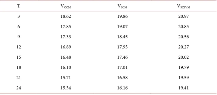
[image:16.595.193.554.547.705.2]

We then allow current product value to vary within a range (thus create a full list of ITM, ATM, and OTM projects) while development duration T varies at the same time. It is interesting to note that the relation between “competition erosion effect” and “val-ue increase effect” varies with project moneyness. In Table 8, when NPD projects are out-of-the-money, “value increase effect” dominates; when investment duration leng-thens, NPD values by all three models increase. However, for in-the-money NPD Table 7. Impact of development duration, T. This table reports NPD values under CCM, CVM and SCSVM models, given different product development duration, T. Simulation uses 1,000 replications. Parameters are defined as in Table 2. All values are in millions.

T VCCM VSCM VSCSVM

3 18.62 19.86 20.97

6 17.85 19.07 20.85

9 17.33 18.45 20.56

12 16.89 17.93 20.27

15 16.48 17.46 20.02

18 16.10 17.01 19.79

21 15.71 16.58 19.59

projects, “competition erosion effect” dominates. This suggests competition intensifies when underlying innovation becomes more profitable.

5.2.4. Project Uncertainty

Project uncertainty comes from two sources, namely, competition uncertainty and un-certainty associated with the product under development. The essence of real option li-terature is that uncertainty creates value (Trigeorgis [2]; Amram and Kulatilaka [5]). Therefore the values of the investment opportunity will increase when project uncer-tainty increases.

[image:17.595.194.555.277.499.2]

Consistent with real option literature, Table 9 suggests that the values of NPD pro- jects increase as competition volatility and the level of project uncertainty increase. Product values estimated with SCSVM are higher than those obtained from CVM and Table 8. Impact of current product value, S(0), and development duration, T.

S(0) T = 6 Months T = 12 Months T = 15 Months

VCCM VCVM VSCSVM VCCM VCVM VSCSVM VCCM VCVM VSCSVM

70 0.01 0.02 0.19 0.13 0.16 0.46 0.22 0.26 0.58

80 0.21 0.26 0.98 0.71 0.81 1.57 0.94 1.06 1.79

90 1.31 1.54 3.09 2.34 2.61 3.87 2.69 2.97 4.48

100 4.47 5.02 7.48 5.54 6.06 8.46 5.85 6.34 8.80 110 10.16 11.09 13.40 10.47 11.26 13.75 10.51 11.24 13.85 120 17.85 19.07 20.85 16.89 17.93 20.27 16.48 17.46 20.02 130 26.62 28.04 29.29 24.37 25.63 27.71 23.46 24.65 27.06 140 35.84 37.41 38.31 32.51 33.95 35.79 31.12 32.48 34.73 150 45.20 46.90 47.63 41.02 42.61 44.27 39.20 40.72 42.83 160 54.61 56.42 57.09 49.72 51.44 53.00 47.52 49.18 51.20 170 64.02 65.95 66.62 58.52 60.36 61.87 55.98 57.76 59.75

Table 9. Impact of project uncertainty*.

σδ VCVM VSCSVM σσ VCVM VSCSVM

0.35 17.91 20.23 0.35 17.93 19.96

0.40 17.91 20.24 0.40 17.93 20.05

0.45 17.92 20.25 0.45 17.93 20.10

0.50 17.93 20.27 0.50 17.93 20.27

0.55 17.94 20.30 0.55 17.93 20.30

0.60 17.96 20.33 0.60 17.93 20.37

0.65 17.97 20.36 0.65 17.93 20.45

0.70 17.99 20.40 0.70 17.93 20.54

[image:17.595.193.551.532.690.2]

CCM, and value difference increases as volatility becomes higher. Also, the marginal contribution of SCSVM increases as uncertainty associated with competition, σ_{δ, and}

with product, σσ, increase. This is consistent with the fact that the marginal

contribu-tion of SCSVM comes from added uncertainty recognized.

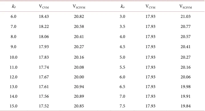
5.2.5. Adjustment Speed, kδ and kσ

Adjustment rates kδ and kσ determine the average time needed to absorb random

shocks generated by changes in competition and product uncertainty. Table 10 indi-cates that when it takes less time to absorb a shock from either source, project values tend to decrease. High levels of kδ imply that competition is more intense. Increased

competitive activities tend to devour more product value, making NPD values low. In-crease in kσ, on the other hand, suggests shorter windows of opportunities opened by

unexpected changes in project uncertainty. As profitable investment opportunities dis-appear quickly, the value of projects tends to be lower.

The marginal contribution of SCSVM over CCM/CVM increases with kδ. The value

differences between SCSVM and CCM/CVM is $3.69 million and $2.36 million, respec-tively, at kδ = 6.0, but rise to $4.05 million and $3.33 million when kδ is 6.0. The result

suggests that the importance of uncertainty to value creation strengthens as more value is devoured by competition. The marginal contribution of SCSVM decreases with kσ.

High kσ value implies shorter windows of opportunities opened by project uncertainty;

consequently reducing the advantage of SCSVM over CCM and CVM.

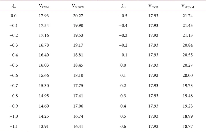
5.2.6. Investor Risk Aversion

Prices of risk, λδ and λσ, represent prices developing firms would be willing to pay to

[image:18.595.194.554.495.690.2]

reduce uncertainty associated with competition erosion and changing product volatility. They also measure levels of risk aversion: when developing firms are more risk-averse, they would accept a higher risk premium, resulting in higher values for λδ and λσ.

Table 10. Impact of rate of adjustment, kδ and kσ*.

kδ VCVM VSCSVM kσ VCVM VSCSVM

6.0 18.43 20.82 3.0 17.93 21.03

7.0 18.22 20.58 3.5 17.93 20.77

8.0 18.06 20.41 4.0 17.93 20.57

9.0 17.93 20.27 4.5 17.93 20.41

10.0 17.83 20.16 5.0 17.93 20.27

11.0 17.74 20.08 5.5 17.93 20.16

12.0 17.67 20.00 6.0 17.93 20.06

13.0 17.61 20.94 6.5 17.93 19.98

14.0 17.56 20.89 7.0 17.93 19.91

15.0 17.52 20.85 7.5 17.93 19.84

Varying λδ and λσ allows us to examine the effect of firms’ risk altitudes towards NPD

valuations.

Notice that competition erosion represents value outflows. As competitors erode the value of the product, they simultaneously bear part of a product’s risk. Consequently competition erosion represents risk sharing. To developing companies, an increase in competition erosion reduces the risk they eventually bear; therefore risk premium re-quested for competition erosion is negative, i.e. developing firms get paid by competi-tors to reduce part of a project’s risk.

Table 11 indicates that when investors and developing firms become more risk- averse, they tend to depress the value of the NPD projects. Risk aversion makes devel-oping firms less willingly to take risk. Because uncertainty is a major source of value creation under the real option approach, we observe a decrease (increase) in project value and a reduced (increased) marginal contribution by SVSCM, as firms are more risk averse (risk prone).

6. Conclusion

[image:19.595.194.553.464.693.2]

We develop a stochastic volatility real option model to value NPD projects that carry managerial flexibility to abandon the project if upon completion, product value falls below the required development cost. Real option theory suggests uncertainty is im-portant to value creation under dynamic management. We explicitly consider the sto-chastic nature of competition erosion and changing project uncertainty across devel-opment stages. We derive a close-form solution under a simplifying assumption of in-dependence between product development uncertainty and other stochastic processes considered in the model. We then solve the full-scale model numerically with Monte Table 11. Impact of price of risk, λδ and λσ*.

λδ VCVM VSCSVM λσ VCVM VSCSVM

0.0 17.93 20.27 −0.5 17.93 21.74

−0.1 17.54 19.90 −0.4 17.93 21.43

−0.2 17.16 19.53 −0.3 17.93 21.13

−0.3 16.78 19.17 −0.2 17.93 20.84

−0.4 16.40 18.81 −0.1 17.93 20.55

−0.5 16.03 18.45 0.0 17.93 20.27

−0.6 15.66 18.10 0.1 17.93 20.00

−0.7 15.30 17.75 0.2 17.93 19.73

−0.8 14.95 17.41 0.3 17.93 19.48

−0.9 14.60 17.06 0.4 17.93 19.23

−1.0 14.25 16.74 0.5 17.93 18.99

−1.1 13.91 16.41 0.6 17.93 18.77

Carlo simulation. Our result is consistent with real option theory. We find a significant undervaluation bias if uncertainties association with competition and changing project volatility are ignored. We examine the marginal contribution (therefore the size of un-dervaluation bias) of our stochastic volatility with stochastic competition model. We find undervaluation bias is more severe when 1) The NPD project is either out-of-the- money or at-the-money; 2) when development duration lengthens; 3) when competi-tion is more intense; 4) when the window of profitable opportunity shortens; and 5) when developing firms are more risk-prone.

References

[1] Trigeorgis, L. and Mason, S.P. (1987) Valuing Managerial Flexibility. Midland Corporate Finance Journal, 5, 14-21.

[2] Trigeorgis, L. (1996) Real Options: Managerial Flexibility and Strategy in Resource Alloca-tion. MIT Press, Cambridge, MA.

[3] Myers, S.C. (1977) Determinants of Corporate Borrowing. Journal of Financial Economics, 5, 147-175. https://doi.org/10.1016/0304-405X(77)90015-0

[4] Kester, W.C. (1984) Today’s Options for Tomorrow’s Growth. Harvard Business Review, 62, 153-165.

[5] Amram, M. and Kulatilaka, N. (1999) Real Options: Managing Strategic Investment in an Uncertain World. Oxford University Press, Oxford.

[6] Caballero, R.J. (1991) On the Sign of the Investment-Uncertainty Relationship. American Economic Review, 81, 279-288.

[7] Kulatilaka, N. (1993) The Value of Flexibility: The Case of a Dual-Fuel Industrial Steam Boiler. Financial Management, 22, 271-280.

[8] Baldwin, C.Y. and Clark, K.B. (2000) Design Rules: The Power of Modularity. MIT Press, Cambridge, MA.

[9] Baldwin, C.Y. and Clark, K.B. (2002) The Option Value of Modularity in Design. Working Paper, Harvard Business School, Boston.

[10] Booz, A.H. (1980) Management of New Products. Booz, Allen and Hamilton, New York. [11] Mansfield, E.D. (1972) Research and Innovation in the Modern Corporation. W.W. Norton

& Co., New York.

[12] Van der Panne, G., van Beers, C. and Kleinknecht, A. (2003) Success and Failure of Innova-tion: A Literature Review. International Journal of Innovation Management, 7, 306-337. [13] Sahal, D. (1981) Patterns of Technological Innovation. Addison-Wesley, Reading, MA. [14] Nelson, R.R. and Winter, S.G. (1982) An Evolutionary Theory of Economic Change.

Har-vard University Press, Cambridge, MA.

[15] Fahey, L. and Narayanan, V.K. (1986) Macroenvironmental Analysis for Strategic Man-agement. West Publishing, Minnesota.

[16] Contractor, F.J. and Narayanan, V.K. (1990) Technology Development in the Multinational Firm: A Framework for Planning and Strategy. R&D Management, 20, 305-322.

https://doi.org/10.1111/j.1467-9310.1990.tb00720.x

[17] Myers, S.C. and Turnbull, S.M. (2002) Capital Budgeting and the Capital Asset Pricing Model: Good News and Bad News. The Journal of Finance, 32, 321-333.

[18] Brennan, M.J. (1973) An Approach to the Valuation of Uncertain Income Streams. The Journal of Finance, 28, 661-674. https://doi.org/10.1111/j.1540-6261.1973.tb01387.x [19] Paddock, J.L., Siegel, D.R. and Smith, J.L. (1988) Option Valuation of Claims on Real

As-sets: The Case of Offshore Petroleum Leases. The Quarterly Journal of Economics, 103, 479-508. https://doi.org/10.2307/1885541

[20] McDonald, R. and Siegel, D. (1984) Option Pricing When the Underlying Asset Earns a Below-Equilibrium Rate of Return: A Note. The Journal of Finance, 39, 261-265.

https://doi.org/10.1111/j.1540-6261.1984.tb03874.x

[21] McDonald, R. and Siegel, D. (1986) The Value of Waiting to Invest. The Quarterly Journal of Economics, 101, 707-727. https://doi.org/10.2307/1884175

[22] Majd, S. and Pindyck, R.S. (1987) Time to Build, Option Value, and Investment Decisions.

Journal of Financial Economics, 18, 7-27. https://doi.org/10.1016/0304-405X(87)90059-6 [23] Trigeorgis, L. (1993) The Mature of Option Interactions and the Valuation of Investments

with Multiple Real Options. The Journal of Financial and Quantitative Analysis, 28, 1-20. https://doi.org/10.2307/2331148

[24] Brennan, M.J. and Schwartz, E.S. (1985) Evaluating Natural Resource Investments. The Journal of Business, 58, 135-157. https://doi.org/10.1086/296288

[25] Kensinger, J. (1987) Adding the Value of Active Management into the Capital Budgeting Decision. Midland Corporate Finance Journal, 5, 31-42.

[26] Myers, S.C. and Majd, S. (1987) Abandonment Value and Project Life. Advances in Futures and Options Research, 4, 1-21.

[27] Chen, S.S., Ho, K.W., Ik, K.H. and Lee, C.F. (2003) The Valuation of New Product Intro-ductions under Uncertain Competition: A Real Option Approach. Advances in Financial Planning and Forecasting, 11, 23-43.

[28] Schwartz, E.S. (2004) Patents and R&D as Real Options. Economic Notes, 33, 23-54. https://doi.org/10.1111/j.0391-5026.2004.00124.x

[29] Chung, K.H. and Charoenwong, C. (1991) Investment Options, Assets in Place, and the Risk of Stocks. Financial Management, 20, 21-32.

[30] Miles, J.A. (1986) Growth Options and the Real Determinants of Systematic Risk. Journal of Business Finance and Accounting, 13, 95-105.

https://doi.org/10.1111/j.1468-5957.1986.tb01175.x

[31] Fama, E.F. and French, K.R. (1988) Commodity Futures Prices: Some Evidence on Forecast Power, Premiums and the Theory of Storage. TheJournal of Business, 60, 55-73.

https://doi.org/10.1086/296385

[32] Fama, E.F. and French, K.R. (1988) Business Cycles and the Behavior of Mental Prices. The Journal of Finance, 43, 1075-1093. https://doi.org/10.1111/j.1540-6261.1988.tb03957.x [33] Gilson, R. and Schwartz, E.S. (1990) Stochastic Convenience Yield and the Pricing of Oil

Contingent Claims. The Journal of Finance, 45, 959-976. https://doi.org/10.1111/j.1540-6261.1990.tb05114.x

[34] Demers, M. (1991) Investment under Uncertainty, Irreversibility and the Arrival of Infor-mation Over Time. The Review of Economic Studies, 58, 333-350.

https://doi.org/10.2307/2297971

[35] Bjerksund, P. and Ekern, S. (1995) Contingent Claims Evaluation of Mean-Reverting Cash Flows in Shipping. In: Trigeorgis, L., Ed., Real Options in Capital Investment: Models,

Strategies, and Applications, Greenwood Publishing Group, Connecticut, 207-219.

of Asset Prices. Econometrica, 52, 363-384. https://doi.org/10.2307/1911241

[37] Cox, J.C. and Ross, S.A. (1976) The Valuation of Options for Alternative Stochastic Pro- cesses. Journal of Financial Economics, 3, 145-166.

https://doi.org/10.1016/0304-405X(76)90023-4

[38] Stein, E.M. and Stein, J.C. (1991) Stock Price Distributions with Stochastic Volatility: An Analytic Approach. The Review of Financial Studies, 4, 727-752.

https://doi.org/10.1093/rfs/4.4.727

[39] Boyle, P.P. (1977) Options: A Monte Carlo Approach. Journal of Financial Economics, 4, 323-338. https://doi.org/10.1016/0304-405X(77)90005-8

[40] Teisberg, E.O. (1995) Methods for Evaluating Capital Investment Decisions under Uncer-tainty. In: Trigeorgis, L., Ed., Real Options in Capital Investment: Models, Strategies, and Applications, Greenwood Publishing Group, Connecticut, 31-45.

[41] Takeuchi, H. and Nonaka, I. (1986) The New New Product Development Game. Harvard Business Review, 64, 137-146.

[42] Stalk, G.J. (1984) Time—The Next Source of Competitive Advantage. Harvard Business Re-view, 66, 41-52.

[43] Millson, M.R., Raj, S.P. and Wilemon, D. (1992) A Survey of Major Approaches for Accele-rating New Product Development. The Journal of Product Innovation Management, 9, 53-69. https://doi.org/10.1111/1540-5885.910053

[44] Day, G.S. and Robin, W. (1988) Assessing Advantage: A Framework for Diagnosing Com-petitive Superiority. Journal of Marketing, 52, 1-20. https://doi.org/10.2307/1251261 [45] Duffie, D. (2010) Dynamic Asset Pricing Theory. Princeton University Press, Princeton. [46] Karatzas, I. and Steven S. (2012) Brownian Motion and Stochastic Calculus. Springer

Appendex A

To owner (i.e. the firm) of the new product, competition erosion creates a dividend-like value outflow. Upon product completion, firm obtains spot new product value. Assume there exists a contract F, which requires the transfer of completed new product to con-tract owner upon product completion. Under a risk-neutral economy, future payment streams from these two positions are identical, therefore values of the contract and NPD project must be the same.

Donate F as the value of the contract. By construction, it should be the function of time t, new product value S t

( )

, product uncertainty σ

( )

t , and the competition

ero-sion δ

( )

t , i.e. F t

( )

= F S t

( ) ( )

,δ t ,σS

( )

t t, . On the maturity date, holder of the contract agrees to exchange it for the completed NPD project. Therefore the boundary condition for the contract could be represented as:

(

, , _S,

)

( )

F S δ σ T =S T (A.1)

with a deterministic continuous sample path of σS, contract value with boundary

condition specified in (A.1) is:

(

)

(

)

e , , , , , , d

T rT

T T T

F K F K p F kσ k rδ α β σ σδ F

∞ −

Θ = −

∫

(A.2)

where dP

( )

⋅ is time T value distribution of the contract condition on given sample

path of σ_Θ.

It can be shown (Cox, Ingersoll and Ross [36], Theorem 3) that the value of the con-tract on NPD project must satisfy the following partial differential equation:

(

)

(

)

2 2 2

1 1

2 2

0

SS S S S

t

F S F F S F S r

F k F rF

δδ δ δ δ δ

δ δ δ δ

σ σ ρ σ σ δ

α δ λ σ

Θ+ + Θ + −

+ _ − − _− − = (A.3)

with boundary condition given in (A.1).

Duffie [45] and Karatzas and Shrev [46] demonstrated that solution to Equation (A.3) with boundary condition (A.1) is given as:

(

)

( )

( ) ( )

(

)

( ) 2 2 2 2 2 1 e

, , exp

1 e

2

1 e

4

k T t t

k T t

S

k T t

F S t S t

k

T t k k k

k k k k δ δ δ δ δ

δ δ δ δ δ δ δ

δ δ δ δ δ δ δ σ

α λ σ ρ σ σ

σ − − − − Θ − −   −  = −     −    − − − − +           +    ₋  _ −           (A.4)

described in (2)* and (4)*, instantaneous value change of the contract is:

(

)

(

)

2 2 2

1 1

d

2 2

d d d

SS S S S

S S

F F S F F S F S r

F k F t F S F

δδ δ δ δ δ

δ δ δ δ τ δ δ δ

σ σ ρ σ σ δ

α δ λ σ σ ω σ ω

Θ Θ Θ  = + + + −   + _ − − _−  + +  (A.5) Denote:

( )

1 e k (T t) A t k δ δ − − −

= _(A.6)

with (A.4) and (A.6), (A.5) can be simplified as:

( )

dF =rF td +Fσ ω_Θd _S−FA t σ ω_δd _δ (A.6a) Since dωS and dωδ are normally distributed with mean zero and variance dt, it is

straightforward that Fσ ωΘd _S −FA t

( )

σ ωδd δ is normal distributed with zero mean

and variance 2

(

)

, , , ,

F δ Sδ k tδ

σ σ σ ρ

Θ .

Denote:

(

)

2 2

( )

2

( )

, , , , 2

F δ Sδ k tδ δA t δ SδA t

σ σ σ ρ

Θ =

σ

Θ+

σ

−

σ σ ρ

Θ (A.6b)

(A.6a) could be simplified to:

dF =rF td +Fσ ωFd F (A.7)

It is obvious that change in contract value dF has a log-normal distribution, i.e.

( )

(

2

)

lnF t N rt,σ_Ft .

The resulting distribution of the contract value at time T is given by:

(

)

( )

(

2

)

2

0 2 log 0.5* 2 , 1 , e 2π T F F

S S r T

T T T F T L S t S σ σ σ σ  _{− −}      −

Θ = (A.8)

with σF defined as in (A.6b).

Appendix B

We follow Stein and Stei [38] to derive the exact distribution of NPD value at time T. Define x=log

(

ST S0

)

−rT and f S

(

T,σΘ

)

=S p S kT

(

T σ,k rδ, , , ,α β σ σσ, δ

)

, where

( )

T

p S ⋅ is NPD value distribution at time t. Using time T distribution of NPD value

(11) as well as (A.8), f S

(

_T,σ_Θ

)

is expressed as:

(

)

(

) ( )

( )

2 2 2 0.5* 2

, , d

1

e d

2π

F F

T T T T

x T

T T F

f S S L S m

m t

σ σ

σ σ σ σ

σ σ

σ

Θ Θ Θ Θ

 +    − Θ Θ = =

∫

∫

(B.1)

( )

( )

( )

(

)

2 2 2 0.5* 2 2 2 1

e e d d

2π exp d 2 F F x T T ix T F F T

g m x

t

T

m i

σ

σ ξ

ξ σ σ

σ σ

σ ξ ξ σ

 +    − Θ Θ Θ Θ       =           = _− + _  

∫

∫

∫

(B.2)

Using definition in (A.6b), 2

F

σ can be expressed as:

(

)

( )

2

( )

(

)

2 2 2

, , , , 1

F δ Sδ k Tδ δ SδA T δA T Sδ

σ σ σ ρ

Θ =

σ

Θ−

σ ρ

 +

σ

−

ρ

And (B.2) can be re-expressed as:

( )

(

2

)

( )

(

2

)

exp * 2

g

ξ

= _−

ξ

+i

ξ

B T _ I_

ξ

+i

ξ

T _ (B.3) where

( )

2

( )

(

2

)

1 S 2

B T =_

σ

δA T −

ρ

δ T_ and I

( )

⋅ is defined as in Stein and Stein [42] (p. 748).

Apply Fourier inversion formula to (B.3) to get:

(

) ( )

1

(

2

)

( )

(

2

)

, 2π e exp d

2

ix T

T f S σ_Θ = − − ξ _− ξ +iξ B T I_ ξ +iξ _ ξ

  

∫

(B.4)

Now make the change of variables of ξ η= −i 2, and recall that x=log

(

ST S0

)

−rT and f S

(

_T,σΘ

)

=S p S k_T

(

_T σ,k rδ, , , ,α β σ σσ, δ

)

, NPD value distribution (11) is given

by:

(

)

( )

(

)

(

2

)

( )

(

)

( )

0

2 0.25 *

1 1.5 2.5 log

, , , , , ,

0.25

2π e e e d

2

T

T

B T _{i S S rT}

rT T

p S k k r

T

S I

σ δ σ δ

η _η

η

α β σ σ

η η ∞ − + − − − − =−∞  +    =    

∫

Appendix C

A Simplified Solution

In this section, we derive a closed-form solution under the assumption that NPD vola-tility follows a deterministic process.

Assume σσ = 0. Partial deferential Equation (6) becomes

(

)

(

)

2 2 2

1 1

2 2

0

SS S S S S S

t

B S B B S B S r

B k B rB

δδ δ δ δ δ σ

δ δ δ δ

σ

σ

ρ σ σ

δ

α δ

λ σ

+ + + −

+ _ − − _− − = (C.1)

Solution to Equation (C.1), with the boundary condition (5), admits the following special representation (Duffi [45]; Karatzas and Shreve [46]):

(

)

_{( )}

(

)

(

)

(

) ( )

( )

* *

0 0

0 0 1 2

, , 0 e d , , , , ,

, , 0 e

rT

T T

S T K

rT

B S S K G k k r

F S N d K N d

σ δ δ

δ α β σ

δ ∞ − = − = − = −

∫

_(C.2)