L e a r ni n g c o s t-s e n si tiv e B ay e si a n
n e t w o r k s vi a d i r e c t a n d in di r e c t
m e t h o d s
N a s h n u s h , E a n d Vad e r a , S
h t t p :// dx. d oi.o r g / 1 0 . 3 2 3 3 /I CA-1 6 0 5 1 4
T i t l e
L e a r n i n g c o s t-s e n s i tiv e B ay e si a n n e t w o r k s vi a d i r e c t a n d
in di r e c t m e t h o d s
A u t h o r s
N a s h n u s h , E a n d Vad e r a , S
Typ e
Ar ticl e
U RL
T hi s v e r si o n is a v ail a bl e a t :
h t t p :// u sir. s alfo r d . a c . u k /i d/ e p ri n t/ 3 8 5 0 8 /
P u b l i s h e d D a t e
2 0 1 6
U S IR is a d i gi t al c oll e c ti o n of t h e r e s e a r c h o u t p u t of t h e U n iv e r si ty of S alfo r d .
W h e r e c o p y ri g h t p e r m i t s , f ull t e x t m a t e r i al h el d i n t h e r e p o si t o r y is m a d e
f r e ely a v ail a bl e o nli n e a n d c a n b e r e a d , d o w nl o a d e d a n d c o pi e d fo r n o
n-c o m m e r n-ci al p r iv a t e s t u d y o r r e s e a r n-c h p u r p o s e s . Pl e a s e n-c h e n-c k t h e m a n u s n-c ri p t
fo r a n y f u r t h e r c o p y ri g h t r e s t r i c ti o n s .
Integrated Computer-Aided Engineering 24 (2017) 17–26 17
DOI 10.3233/ICA-160514 IOS Press
Learning cost-sensitive Bayesian networks
via direct and indirect methods
Eman Nashnush and Sunil Vadera
∗The School of Computing, Science and Engineering, University of Salford, Manchester, UK
Abstract.Cost-sensitive learning has become an increasingly important area that recognizes that real world classification
prob-lems need to take the costs of misclassification and accuracy into account. Much work has been done on cost-sensitive decision tree learning, but very little has been done on cost-sensitive Bayesian networks. Although there has been significant research on Bayesian networks there has been relatively little research on learning cost-sensitive Bayesian networks. Hence, this paper explores whether it is possible to develop algorithms that learn cost-sensitive Bayesian networks by taking (i) an indirect ap-proach that changes the data distribution to reflect the costs of misclassification; and (ii) a direct apap-proach that amends an existing accuracy based algorithm for learning Bayesian networks.An empirical comparison of the new approaches is carried out with cost-sensitive decision tree learning algorithms on 33 data sets, and the results show that the new algorithms perform better in terms of misclassification cost and maintaining accuracy.
Keywords: Cost-sensitive classification, Bayesian learning, decision trees
1. Introduction
The ability to learn classifiers has been one of the major success stories of AI [13,36], with a wide range of methods such as neural networks, decision tree in-duction, support vector machines, and Bayesian net-works utilised in many real world applications such as fraud detection, assessing credit, cyber security and medical diagnosis [1,24,37].
Early machine learning algorithms, now termed cost-insensitive learning algorithms, focused on maxi-mizing accuracy but did not take any type of costs into account [20]. Several authors have noted that this is not adequate for practical applications [7,18]. For ex-ample, in medical diagnosis applications, the cost of a false positive error includes unnecessary treatment and unnecessary worry while the cost of a false negative error includes postponed treatment or failure to treat and death or injury [28]. In fraud detection applica-tions, a false positive error can lead to resources being
∗Corresponding author: Sunil Vadera, The School of
[image:2.595.309.526.458.503.2]Comput-ing, Science and EngineerComput-ing, Salford University, Manchester, UK. E-mail: [email protected].
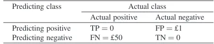
Table 1
A cost matrix for two-class problems
Predicting class Actual class
Actual positive Actual negative Predicting positive TP=0 FP=£1 Predicting negative FN=£50 TN=0
wasted investigating non-frauds and reducing the ben-efits; while a false negative error such as a failure to detect fraud could be very expensive [25].
Hence, in recent years, a significant level of atten-tion has been paid to cost-sensitive learning, including making accuracy-based learners cost-sensitive [18]. Cost-sensitive learning algorithms take costs into con-sideration and aim to minimize expected cost [16]. The following example illustrates the use of a cost matrix together with some of the key ideas. Table 1 presents an example cost matrix, whereCi,j is the cost of pre-dicting an example to be in class i when it is actually in class j [9,34].
A classification scheme, when applied to some data, will lead to outcomes that are correct or incorrect, re-sulting in what is known as a confusion matrix. For example, suppose we have two different classifiers, C1 and C2, induced by two different learning
algo-ISSN 1069-2509/17/$35.00 c2017 – IOS Press and the author(s). All rights reserved
Table 2a
Outcomes of decision tree classifier (J48) on Hepatitis test set
Predicting class Actual class Actual die Actual live
Predicting die 4 7
Predicting live 5 25
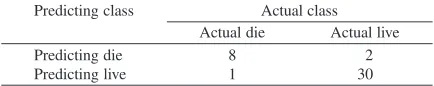
Table 2b
Outcomes of Bayesian network classifier on Hepatitis test set
Predicting class Actual class Actual die Actual live
Predicting die 8 2
Predicting live 1 30
rithms; say a Decision tree classifier and a Bayesian network classifier. Applying these classifiers to a Hep-atitis dataset and evaluating the supplied test set in the model may give the results in Tables 2(a) and 2(b) re-spectively.
Given the outcomes in Tables 2(a) and 2(b), we can compute the accuracy and misclassification costs of the two classifiers by using the following measures:
Accuracy= No. of correct examples
Total number of examples (1)
Cost=
N
j=0
No Missclassifiedj∗Costj (2)
WhereNis the number of classes, No Misclassifiedj is the number of classj examples that are misclassi-fied, and Costj is the cost of misclassifying examples of classj. Using these equations, we obtain the follow-ing accuracies and costs for the decision tree (DT) and the Bayesian network (BN):
DT Accuracy=70.73% DT Misclassification cost=257 BN Accuracy=92.68% BN Misclassification cost=52
Thus, in this example, applying the Bayesian net-work classifier will entail less cost than applying the Decision tree classifier on the Hepatitis dataset. The task of cost-sensitive learning is to induce classifiers that minimize cost. Most of the work on inducing clas-sifiers has focused on decision tree learning and, to the best knowledge of the authors, there has been no at-tempt to assess whether the use of Bayesian networks can produce better cost-sensitive classifiers than deci-sion tree induction. Hence, this study aims to explore the use of Bayesian networks (BNs) for cost-sensitive classification.
The study builds upon a paper presented at the First International Conference on Soft Computing and Data Mining (SCDM-2014) in which the authors presented the initial results from using a sampling method [21]. In this paper, the authors present a new direct approach to learn cost-sensitive Bayesian networks, and present new results in comparison to the use of sampling.
This paper is organized as follows. Section 2 pres-ents some background on Bayesian networks. Sec-tion 3 provides a number of definiSec-tions and a sum-mary of related work and background information on cost-sensitive learning algorithms. Section 4 presents two alternative approaches for learning cost-sensitive Bayesian networks: one by using a direct approach that amends an algorithm and a second that uses an indirect approach that uses sampling to amend the distribution of the training data to reflect costs of misclassification as previously presented in [21]. Section 5 shows the re-sults obtained by carrying out an empirical evaluation on data from the UCI repository [3]. Finally, Section 6 provides a conclusion and summary of the main con-tribution of this paper.
2. Background on Bayesian networks
A Bayesian network (BN) can be used as a classi-fier by computing the posteriori probability of a set of labels given the observable features [24]. According to Neapolitan [22] there are two aspects to construct-ing a BN:(i) learn the graphical structure(topology), that is the relationships between the variables; and(ii) learn the parameters(conditional probability estima-tion) which quantify the extent of the relationships.
[image:3.595.68.285.219.262.2]E. Nashnush and S. Vadera / Learning cost-sensitive bayesian networks via direct and indirect methods 19
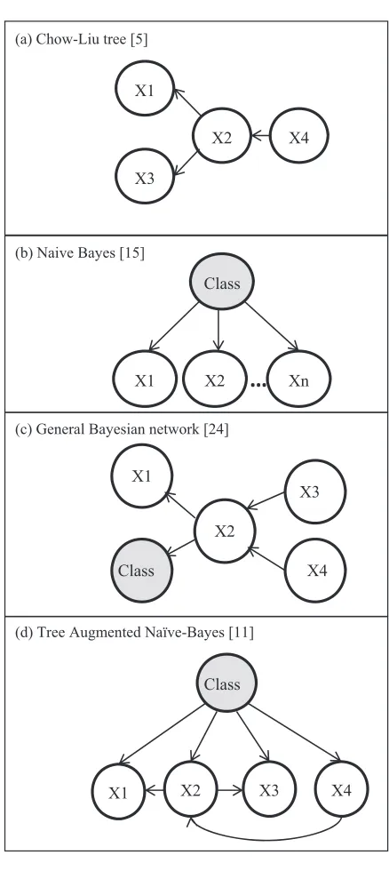
Bayesstructure, where all attributes are represented as independent nodes that have one parent (class node). A Naive Bayes classifier, as shown in Fig. 1(b), as-sumes conditional independence of the features given the class. Naive Bayes is easy to construct and it has been used as a classifier for many years, especially where the features are not strongly correlated. More re-cently, in 1997, Friedman et al. [11] developed a nat-ural extension to the Naive Bayes classifier and the Chow-Liu algorithm, where they introduce the Tree Augmented Naive Bayes(TAN) structure. In contrast to Naive Bayes, where the assumption is that all attributes are independent, in a TAN all attributes are condition-ally independent given the value of the class. Thus in a TAN, the correlations between attributes can be cap-tured by adding additional edges between attributes, as shown in Fig. 1(d).
Learning network structure requires searching for the best network according to a score. Many scor-ing criteria have been proposed such as: theBayesian Dirichlet scoring function (BD)[14], theBayesian In-formation Criterion (BIC)[29], theMinimum Descrip-tion Length (MDL)[27], and theAkaike’s Information Criterion (AIC) [2]. All these measures have different characteristics and the reader can refer to [12] for de-tails. The MDL measure is used in the algorithm we adapt and is described below.
Let us assume thatB =<G, O>is a Bayesian net-work, where G is an acyclic graph and O denotes the parameters consisting of the conditional probabilities.
LetDbe a training set, then the MDL score can be defined by [11,22]:
MDL(B|D) = 1/2logN∗ |B| −LL(B|D) (3)
There are two parts to this definition. The first part,1/2 log N *|B|denotes the number of bits required to rep-resent the network, where N is the number of instances;
|B|is the number of parameters in the network; and1/2 log N represents the number of bits that are used for each parameter. The second part, LL(B|D), represents the log likelihood of B given D, and denotes how many bits are needed to describe the data D based on the probability distribution PBand is given by [11,19,22]:
LL(B|D) =
N
i=1
PB(ui)∗log(PB(ui)) (4)
In particular, the highest log likelihood refers to the closest model B with the probability distribution of the data D. The MDL score focuses on combining the length of the network description and encoding the data to be minimized.
X3 X4
X1 X2
Class X2
X4 X1
Class
X3
X2 Xn
X1
Class
…
X3
X4 X1
X2
(d) Tree Augmented Naïve-Bayes [11] (a) Chow-Liu tree [5]
(b) Naive Bayes [15]
[image:4.595.308.527.105.595.2](c) General Bayesian network [24]
Fig. 1. Bayesian structures.
3. An overview of approaches to cost-sensitive learning
As illustrated by the example in Section 1, the aim of a cost-sensitive classifier is to minimize the expected cost of classification [9].
cat-egories: Black Box andTransparent Box. Black box methods use a closed box without changing the clas-sifier behavior and can work for any clasclas-sifier. On the other hand, transparent box methods require knowl-edge of the particular learning algorithm and are based on changing the algorithm to include costs. Ling and Sheng [16] use different terms such asdirect method, andindirect methods.
Adirect method,introduces misclassification costs into algorithms such as cost sensitive decision trees [4, 8,17,23]. On the other hand,indirect methodsuse tech-niques such as Sampling [31,34], Relabelling [7,33], Weighting [32], and Thresholding [9,30]. These meth-ods can be applied before or after applying an exist-ing accuracy based classifier. The followexist-ing sections describe the application of direct and indirect meth-ods to produce cost-sensitive decision tree learning al-gorithms. There are numerous methods that could be described and we focus on just a couple to illustrate the main ideas that we use later in Sections 4 and 5. Readers interested in other methods are referred to a comprehensive survey carried out by Lomax and Vadera [18].
3.1. Cost-sensitive direct learning methods
A key step in decision tree learning is to select the criteria used for the next node of the decision tree and to split the data. Early decision tree induction algo-rithms that focused on accuracy used a measure based on information theory to select the splitting criteria. For example, ID3, and C4.5 [26] are based on calculing the gain in information achieved by each of the at-tributes if these were chosen for the split and choosing the attribute which maximizes this gain:
InfoA=E(D)−E(A) (5)
Where:
E(D) =
c∈C
−NcN ∗log2Nc
N
E(A) =
a∈A
P(a)∗ c∈C
−P(a|c)∗log2P(a|c)
Where,a∈Aare the values of attribute A, andc∈
Care the class values.
Thus, an obvious way of adapting these algorithms is to amend this measure to take account of costs. For example, Breiman et al. [4] modify the class probabil-ities that are used in the information gain measure, and exchange that probability with the altered probability
as shown in Eq. (6), where the probability for a class
iis weighted by the relative cost of misclassifying an example of classi(Cost ratioi).
Altered Probabilityi=Cost ratioi∗
Ni N
(6)
Where, forkclasses:
Cost ratioi= costi
Σk jcostj
For example, for the cost matrix in Table 1, the cost ratio for the positive class is 50/51, while, the cost ratio for the negative class is 1/51. Also, Ni is the number of examples in classi, whileN is the total number of examples.
3.2. Cost-sensitive indirect learning method
Indirect methods do not change the learning process of a classifier and instead use it as a black box. As an example, consider one the earliest indirect methods, called MetaCost [7]. In this method, an accuracy based learner is used on several samples of the data, each re-sulting in a decision tree. The rere-sulting trees are used to predict the class of each example, and then used to predict the class that minimises the cost, which in turn is used to relabel the examples. The accuracy based learner is then applied on the relabelled data to pro-duce a cost-sensitive decision tree. Another interesting indirect method is Costing [34] which makes use of a result due to Elkan [9] that states a Folk Theorem that the data distribution can be changed to reflect the costs. As Zadrozny et al. [35] state:
“If the new examples are drawn from the old dis-tribution, then optimal error rate classifiers for the new distributions are optimal cost minimizers for data drawn from the original distribution.”
This is presented as the following equation [35]:
D(x, y, c) = C
Ex,y,c∼D[c]D(x, y, c) (7) Where, the new distributionD =factor * Old dis-tribution D;xis instance;y is the class label; and C is the cost according to misclassified instancex. This theorem can be used to create a new distribution from the old distribution by multiplying the old distribution with a factor proportional to the relative cost of each example.
E. Nashnush and S. Vadera / Learning cost-sensitive bayesian networks via direct and indirect methods 21
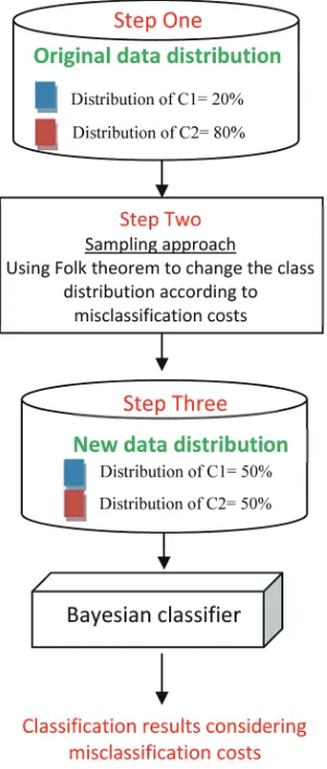
Fig. 2. Changing the data distribution of hepatitis dataset.
0%), and 123 instances in the class “live” (class dis-tribution 80%). Given the imbalance in examples for the two classes, an accuracy based classifier will al-ways be biased to the most common class, that is live, though misclassifying examples of class “die” is more serious. The folk theorem can be used to address this kind of situation. Suppose the misclassification costs are 4:1 for Live: Die respectively. Then the new distri-bution of class die=4*32=128 die (class distribution 50%); and the new distribution of class live=1*123
=123 live (class distribution 50%), as summarised by the steps given in Fig. 2.
4. Development of cost-sensitive Bayesian networks
The direct and indirect methods described above, have been used mainly when developing cost-sensitive
decision tree learners. Section 4.1 describes the use of a direct approach for learning cost-sensitive Bayesian networks and Section 4.2 describes an indirect ap-proach for learning cost-sensitive Bayesian networks.
4.1. Cost-sensitive Bayesian network induction via a direct approach
As described in Section 2, a key step of existing al-gorithms for learning the structure of a Bayesian net-work is to compute the Minimum Description Length (MDL). Hence, by analogy with the approach taken for decision trees, where the information theoretic mea-sure was modified, the modification made to develop our new algorithm is to change the original MDL mea-sure [27], which was described in Section 2 in Eqs (3) and (4).
As with the modification made for decision trees, we make two amendments when learning the structure of a Bayesian network.
First, the Log-likelihood factor that is used in the MDL measure Eq. (4) is amended to take account of costs. The modification made is to multiply each part of the information measurement with the cost propor-tion of a class, resulting in the new LL(B|D) given in Eq. (8).
LL(B|D) =
k
j=1
N
i=1
p(xi, πxi) log2
(8)
p(xi, πxi)
p(πxi)
∗Cost ratioj
Where, M is the number of class labels, N is the num-ber of parent attributes to nodexi,πxirepresents the parents of the attributexiand Cost ratiojis the ratio of the cost of misclassifying class j over the total costs, as described in Section 3.1. Whilep(xi, πxi)represents the probabilities of events in D.
Secondly, the parameters are modified to reflect costs by modifying the conditional probability of each node given its parent. That is, instead of using the Laplace estimator ofP(i), we weight it by the cost ra-tio:
Pclassj(xi|πxi) =Cost ratioj∗ p
(xi, πxi) + 1
p(πxi) +nxi (9)
Where,xiis the node that is connected withπxi(class label, and another parent);nxiis the number of possi-ble values of nodexi.
2
3
4 5
6
CS-BN via D
1. Compute
(nodes) based
2. Build a co each pair node.
3. Use the Maximum Weight Spanning Tree algorithm,
gained ab the cost of 4. Convert th 5. Add the c
(nodes). 6. Learn the
parent by
that includes misclassification costs.
irect approach:
new between e on clas for
mplete undir of attributes
, to maximize the information out the class
misclassific e tree to a dir lass label as
parameters fo
using the new probability estimation conditional
ach pair of a s label, and
each class in the calculation, based on MDL score:
ected graph (nodes) witho
ification weig ation to obtain
ected tree. root for all a
r each node mutual information
a ttributes
include cost proportions
between out class
ghted by n a tree.
attributes
with its
Fig. 3. Cost-Sensitive Bayesian Network Algorithm by direct amendment.
4.2. Cost-sensitive Bayesian networks induction via an indirect approach
This section presents an indirect approach to de-velop cost-sensitive Bayesian networks (CS-BNs) that uses sampling to take account of misclassification costs. The approach used is based on that introduced by Zadrozny et al. [35] and Elkan’s Folk Theorem [9] that was described in Section 3.2. This theorem draws a new distribution from the old distribution, according to cost proportions to change the data distribution and obtain optimal cost-minimization from the original dis-tribution. Figure 4 gives the algorithm we adopt using sampling.
The main steps of this algorithm are:
Step 1: The data are split into a training set and test-ing set. The traintest-ing set uses 75% of the original data, while the testing set uses 25% of the original data.1
Step 2: The distribution of the data is altered to take account of costs. For instance, if the cost of wrongly classifying a sick patient as healthy is £20 and the cost of misclassifying a healthy patient as sick is £2, then the cost ratio of the sick class will be 20/22 =0.90.
1Other ways of splitting the data could, of course be adopted
with-out affecting the principles of the approach.
CS-BN via Indirect approach (Sampling)
1. Divide dataset into 75% of instances for training, and 25% for testing. With the same class distributions.
2. Change the data distribution according to the cost ratio of each class:
3. Learn the TAN structure and its parameters 4. Evaluate the TAN on the original test set
distribution.
Fig. 4. Cost-sensitive Bayesian network algorithm by indirect ap-proach using sampling.
The cost ratios are then used to change the data distri-butions. For example, if a dataset has a class distribu-tions of 50% for each class, when the costs are 1:4, the new proportions for each class will be 20% and 80% respectively. There are different methods that can be used to sample the data to redistribute the data. During our research, we used two methods, under-sampling and over-sampling. Where the new proportion was less than the original proportion, we used under-sampling (without replacement) to delete some of the examples in the frequent class. On the other hand, if the new proportion was greater than the original proportion, we used over-sampling (with replacement) to randomly select new instances which belonged to the rare class, and hence increase the number of examples.
Step 3:Uses Friedman et al.’s [11] cost-insensitive algorithm on the new distribution from step 2.
Step 4:Evaluates the model on the original distribu-tion.
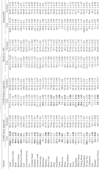
5. Empirical evaluation
This section presents an empirical evaluation of the amended cost-sensitive BN algorithm, and CS-BN using a sampling approach. The evaluation is car-ried out using 33 data sets from the UCI reposi-tory [3] and adopting the 75% training and 25% test-ing methodology. The cost matrix adopts 16 cost ratios [4:1,4:2,4:3,4:4, 3:1,.., 1:4]. The evaluation is carried out with respect to the two methods presented in this paper as well as the following algorithms:
(i) The original TAN learning algorithm [11], to as-sess the extent to which the amendments make a difference.
E. Nashnush and S. Vadera / Learning cost-sensitive bayesian networks via direct and indirect methods 23
0 0.2 0.4 0.6 0.8 1 1.2 1.4 1.6
Misclassification costs
[image:8.595.70.528.133.326.2]CS-BN indirect approach CS-BN direct approach Cost of MetaCost algorithm Cost of BN algorithm
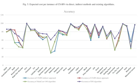
Fig. 5. Expected cost per instance of CS-BN via direct, indirect methods and existing algorithms.
0 20 40 60 80 100 120
Accuracy
Accuracy of CS-BN indirect approach Accuracy of CS-BN direct approach
[image:8.595.70.531.147.537.2]Accuracy of MetaCost+J48 algorithm Accuracy of BN algorithm
Fig. 6. Accuracy of CS-BN via direct, indirect methods and an existing algorithm.
Table 3 presents the results for each of the 33 data sets and highlights the result with the lowest cost for each data set. Figure 5 presents the results of expected costs for each data set in the form of bar charts, and Fig. 6 presents the accuracy across different data sets.
These experiments show that:
(i) The numbers of misclassifications of the rare
class (i.e., more expensive) are always less than the number of misclassifications of the frequent class in all datasets.
[image:8.595.66.531.324.606.2]E. Nashnush and S. Vadera / Learning cost-sensitive bayesian networks via direct and indirect methods 25 imizing costs than the indirect approach in 19
out of the 33 data sets evaluated
(iii) The use of the indirect approach, involving changing the data distributions yields good re-sults on most data; especially if the data are not very highly skewed towards one class.
(iv) The indirect approach performed better in terms of minimizing costs than the direct approach in 14 out of the 33 data sets evaluated.
(v) Overall, both the direct and indirect versions outperform MetaCost+J48, and the original ac-curacy only version in terms of minimizing cost. Both approaches performed better in terms of minimizing costs than MetaCost+J48, and orig-inal BN algorithm in 27 out of the 33 data sets evaluated.
(vi) The accuracy of the cost-sensitive version is similar but slightly less than the original accu-racy based version of TAN, though the level of sacrifice is not as significant as reported in stud-ies that use similar approaches for learning cost-sensitive decision trees [18].
6. Conclusion
Cost-sensitive learning algorithms have received in-creasing attention in most real world applications, though most of the existing studies are devoted to mak-ing decision trees cost-sensitive. Existmak-ing Bayesian network algorithms that are designed to minimize misclassification errors do not take misclassification costs into consideration. Hence, this study has ex-plored whether it is possible to develop cost-sensitive Bayesian networks. Two algorithms were developed by analogy with the strategies used for producing cost-sensitive decision trees: (i) a direct approach that in-volved amending the MDL measure used in construct-ing a network and (ii) an indirect approach, based on sampling to change the distribution of examples to re-flect the costs of misclassification.
The main findings from the empirical evaluation rel-ative to other algorithms are:
– As one would expect, the new algorithms outper-formed the cost-insensitive version of the algo-rithm that learns Bayesian networks.
– The direct approach gives good results on most of the data sets and is also better than the indirect proach on some data sets, while, the indirect ap-proach works very well when the data are not very highly skewed towards one class.
– In our evaluations, both the direct and indirect ap-proaches performed better than MetaCost+J48 in terms of minimizing costs.
In conclusion, application of strategies to induce cost-sensitive decision trees to learn cost-sensitive Bayesian networks have proved to be effective and, in general, lead to more cost-effective classification than the use of decision trees.
Acknowledgements
This paper is an extended and refined version of the paper presented at the First International Confer-ence on Soft Computing and Data Mining (SCDM-2014) reference [21]. The authors are grateful to the re-viewers and editor for their constructive comments that have helped improve the presentation of this paper.
References
[1] M. Ahmadlou and H. Adeli, Enhanced probabilistic neural network with local decision circles: A robust classifier, Inte-grated Computer-Aided Engineering17(3) (2010), 197–210. [2] H. Akaike, A new look at the statistical model identification,
IEEE Transactions on Automatic Control19(6) (1974), 716– 723.
[3] A. Asuncion and D.H. Newman, UCI machine learning repos-itory, https://archive.ics.uci.edu/ml/datasets.html, (2007). [4] L. Breiman, J. Friedman, C.J. Stone and R.A. Olshen,
Classi-fication and regression trees. CRC press, 1984.
[5] C.K. Chow and C.N. Liu, Approximating discrete probabil-ity distributions with dependence trees,IEEE Transactions on Information Theory4(3) (1968), 462–467.
[6] S. Dasgupta, Learning polytrees, InProceedings of the Fif-teenth conference on Uncertainty in artificial intelligence
(1999), pp. 134–141.
[7] P. Domingos, Metacost: A general method for making classi-fiers cost-sensitive, InProceedings of the fifth ACM SIGKDD international conference on Knowledge discovery and data mining, (1999), pp. 155–164.
[8] C. Drummond and R.C. Holte, Exploiting the cost (in) sensi-tivity of decision tree splitting criteria, InICML, (2000), pp. 239–246.
[9] C. Elkan, The foundations of cost-sensitive learning, Inter-national Joint Conference on Artificial Intelligence 17(1) (2001), 973–978.
[10] J.H. Friedman, Data Mining and Statistics: What’s the con-nection?Computing Science and Statistics29(1) (1998), 3–9. [11] N. Friedman, D. Geiger and M. Goldszmidt, Bayesian Net-work Classifiers,Machine Learning29(2-3) (1997), 131–163. [12] N. Friedman and M. Goldszmidt, Learning Bayesian net-works with local structure, InLearning in Graphical Models, Springer Netherlands, (1998), pp. 421–459.
[14] D. Heckerman, A. Mamdani and M.P. Wellman, Real-world applications of Bayesian networks,Communications of the ACM 38(3) (1995), 24–26.
[15] P. Langley, W. Iba and K. Thompson, An analysis of Bayesian classifiers, InProceedings, Tenth National Conference on Ar-tificial Intelligence, Menlo Park, CA: AAAI Press,90, (1992), 223–228.
[16] C.X. Ling and V.S. Sheng, Cost-sensitive learning, In Ency-clopedia of Machine Learning(2010), pp. 231–235. [17] C.X. Ling, Q. Yang, J. Wang and S. Zhang, Decision Trees
with Minimal Costs,ACM International Conference Proceed-ing Series 21st international conference on Machine learn-ing, Banff, Alberta, Canada, Article No. 69, ACM Press New York, NY, USA, (2004).
[18] S. Lomax and S. Vadera, A survey of cost-sensitive decision tree induction algorithms,ACM Computing Surveys (CSUR)
45(2) (2013), 16.
[19] M. Meila and M.I. Jordan, Learning with Mixtures of Trees,
Journal of Machine Learning Research(2000), 1–48. [20] T.M. Mitchell, Does machine learning really work?AI
maga-zine18(3) (1997), 11.
[21] E. Nashnush and S. Vadera, Cost-Sensitive Bayesian Network Learning Using Sampling, InRecent Advances on Soft Com-puting and Data Mining, Springer International Publishing, (2014), pp. 467–476.
[22] R.E. Neapolitan, Learning Bayesian networks, Upper Saddle River: Prentice Hall, (2004).
[23] M.J. Pazzani, C.J. Merz, P.M. Murphy, K. Ali, T. Hume and C. Brunk, Reducing Misclassification Costs, InICML, (1994), pp. 217–225.
[24] J. Pearl, Embracing Causality in Formal Reasoning, InAAAI, (1988), pp. 369–373.
[25] C. Phua, V. Lee, K. Smith and R. Gayler, A comprehensive survey of data mining-based fraud detection research,arXiv preprint arXiv: 1009.6119, (2010).
[26] J.R. Quinlan, Induction of decision trees,Machine Learning
1(1) (1986), 81–106.
[27] J. Rissanen, Modeling by shortest data description, Automat-ica14(5), (1978), 465–471.
[28] R. Santos-Rodríguez, D. García-García and J. Cid-Sueiro, Cost-sensitive classification based on Bregman divergences for medical diagnosis, InMachine Learning and Applications, ICML, (2009), pp. 551–556.
[29] G. Schwarz, Estimating the dimension of a model,The Annals of Statistics6(2) (1978), 461–464.
[30] V.S. Sheng and C.X. Ling, Thresholding for making classi-fiers cost-sensitive, InProceedings of the national conference on artificial intelligence. Menlo Park, CA; Cambridge, MA; London; AAAI Press; MIT Press.21(1) (2006), pp. 476. [31] V.S. Sheng and C.X. Ling, Roulette sampling for
cost-sensitive learning, InMachine Learning: ECML, Springer, (2007), pp. 724–731.
[32] K.M. Thing, An Instance-Weighting Method to Induce Cost-Sensitive Decision Trees,IEEE Transactions on Knowledge and Data Engineering14(3) (2002), 659–665.
[33] I.H. Witten and E. Frank,Data Mining – Practical Machine Learning Tools and Techniques with Java Implementations, Morgan Kaufmann Publishers, (2005).
[34] B. Zadrozny, J. Langford and N. Abe, A simple method for cost-sensitive learning,IBM Technical Report RC22666, (2003).
[35] B. Zadrozny, J. Langford and N. Abe, Cost-sensitive learn-ing by cost-proportionate example weightlearn-ing, InData Min-ing, ICDM, Third IEEE International Conference, (2003), pp. 435–442.