AUTOMATIC DETECTION AND
IDENTIFICATION OF CELLS IN DIGITAL
IMAGES OF DAY 2 IVF EMBRYOS
Marwa Ali Elshenawy
AUTOMATIC DETECTION AND
IDENTIFICATION OF CELLS IN DIGITAL
IMAGES OF DAY 2 IVF EMBRYOS
Marwa Ali Elshenawy
School of Computing, Science and Engineering
University of Salford, Salford, UK
Submitted in Partial Fulfilment of the Requirements of the
i
Table of Contents
Contents... i
Glossary
... viList of Tables
... viiList of Figures
... ixAcknowledgements
... xivDeclaration
...xvAbstract
... xviChapter 1 Introduction ... 1
1.1 Introduction to infertility ...2
1.1.1 Oocyte retrieval...2
1.1.2 Sperm collection ...3
1.1.3 Fertilization ...3
1.1.4 Embryo cleavage...4
1.1.5 Embryo grading ...5
1.1.6 Transferring problem ...10
1.2 The image dataset used in this study ...11
1.3 Aims and objectives ...14
1.4 Thesis structure...15
Chapter 2 Literature survey... 18
2.1 Previous work on cell detection ...18
2.2 Previous work on embryo detection ...20
Chapter 3 Digital Image Processing ... 29
3.1 Image representation ...29
3.2 Image pre-processing ...30
3.2.1 Image brightness and contrast enhancement...30
3.2.2 Histogram equalization ...33
3.2.3 Image smoothing...35
3.2.4 Image segmentation ...40
3.2.4.1 Edge detection...40
3.2.4.2 Thresholding ...44
3.3 Object detection...45
3.3.1 Hough Transform...45
3.3.2 Template matching...47
3.4 Implementing the Image processing algorithms ...49
3.5 Conclusion...49
Chapter 4 Pre-processing of the embryo images... 50
4.1 Introduction ...50
4.2 Magnification compensation ...51
4.2.1 Detection of the ZP ...51
4.2.2 The size of ZP ...54
4.3 Edge detection ...55
4.3.1 Edge setection using basic techniques ...55
4.3.2 Edge detection using a new approach ...56
4.3.3 Edge detection using convolution mask ...59
iii
Chapter 5 Embryo Detection using the Hough Transform ... 61
5.1 Introduction ...61
5.2 Proposed technique...62
5.3 Results of applying Hough Transform ...67
5.4 Results using the Hough Transform. ...78
5.5 Conclusions ...79
Chapter 6 Embryo detection using template matching ... 81
6.1 Introduction ...81
6.2 The proposed algorithm...82
6.2.1 Templates generation ...82
6.2.2 Correlation process ...85
6.3 Results using the SAD and NCC correlation techniques ...89
6.3.1 Considering one peak value ...89
6.3.2 Considering peak values 93 6.4 Summary of template matching results ...97
6.4 Conclusion...98
Chapter 7 Embryo detection using Binary Template Matching ... 99
7.1 Introduction ...99
7.2 The binary template matching technique ...100
7.3 Results for the binary templates matching technique ...102
7.4 Summary of the binary template matching results ...110
Chapter 8 Refining the Binary Template Matching... 112
8.1 Introduction ...112
8.2 Refining the binary template matching results ...113
8.2.1 Applying filters ...113
8.2.2 Applying two templates ...122
8.3 Conclusion...128
Chapter 9 Results and Discussion ... 129
9.1 Introduction ...129
9.2 Summary of Results ...130
9.3 Results for the testing dataset ...134
9.3.1 Applying the algorithm ...134
9.3.2 Results...140
9.4 Classification results...141
9.5 Conclusion...143
Chapter 10 Conclusions... 144
10.1 Summary of the aims and objective and work done ...144
10.2 Summary of the results and findings ...145
v
Bibliography…... 145
Appendix A…... 152
Appendix B…... 154
Appendix C…... 173
Appendix D…... 179
Appendix E…... 187
Appendix F…... 202
Appendix G…... 225
Appendix H…... 226
Appendix I…... 232
Glossary
ART
Assisted Reproductive Technologies
BPS
Border Percentage Sensitivity
ICM
Inner Cell Mass
ICSI
Intra Cytoplasmic Sperm Injection
IPS
Interior Percentage Sensitivity
IVF
In Vitro Fertilization
NCC
Normalized Cross Correlation
SAD
Sum of Absolute Difference
TE
Trophectoderm
vii
List of Tables
Table 1.1 Parameters of embryo quality ... 13
Table 2.1 Mean blastomere sizes of embryos at different cleavage stages (Hnida et al. (2004))...21
Table 2.2 Mean blastomere volume as function of degree of fragmentation (Hnida et al. (2004))...22
Table 2.3 Detection method of the features ...23
Table 2.4 Summary of the survey ...27
Table 5.1 The value of the array ...65
Table 5.2 Values after elimination ...67
Table 5.3 Hough-based technique results ...79
Table 6.1 One peak template matching results ...97
Table 6.2 Multi-peak template matching results ...97
Table 7.1 Binary template matching technique results ...110
Table 8.1 Results when applying median filter...121
Table 8.2 Results when using Hough Transform on filtered images ...122
Table 8.3 Enhanced "AND" technique results ...127
Table 9.1 Hough-based technique results ...130
Table 9.2 One peak template matching results ...131
Table 9.3 Multi-peak template matching results ...131
Table 9.4 Enhanced template matching technique results ...132
Table 9.5 Results when using Hough Transform on filtered imaged...132
Table 9.6 Results when applying median filter...133
Table 9.8 Summary of the results...140
Table 9.9 Classification results ...141
ix
List of Figures
Figure 1.1 Oocyte retrieval ...3
Figure 1.2 ICSI...4
Figure 1.3 Embryo development stages ...4
Figure 1.4 Zygote scoring features ...5
Figure 1.5 Scott's zygote scoring grades ...6
Figure 1.6 Cleaved embryo grading features ...7
Figure 1.7 Blastocyst grading features...9
Figure 1.8 Gardner's system (top) embryo development grading (bottom) ICM and TE grading...10
Figure 1.9 Embryos transfer...10
Figure 2.1 Subjective features of human zygote...23
Figure 3.1 Image representation...29
Figure 3.2 Image histogram ...31
Figure 3.3 Image brightness enhancement (top) original image (middle) image after increasing the brightness (bottom) image after decreasing the brightness ...31
Figure 3.4 Contrast enhancement (a) original image (b) image after contrast enhancement ...33
Figure 3.5 Example of histogram equalisation ...35
Figure 3.6 Neighbourhood (a) 4 neighbours (b) 8 neighbours ...36
Figure 3.7 3x3 masking process...37
Figure 3.8 3x3 mean smoothing mask ...38
Figure 3.10 Effect of median smoothing ...39
Figure 3.11 Different types of edges (a) ideal image (b) digital image (c) abrupt change in grey level (d) ramp change in the grey level (e) first derivative of the ramp. ...41
Figure 3.12 Roberts 2x2 masks...42
Figure 3.13 Sobel 3x3 masks ...43
Figure 3.14 Prewitt 3x3 mask ...43
Figure 3.15 Thresholding using histogram ...44
Figure 3.16 The xy plane and the parametric plane ...45
Figure 3.17 Hough transform of a circle with fixed radius...46
Figure 3.18 Template Matching...48
Figure 3.19 Results of NCC...48
Figure 4.1 Result of detecting the ZP using Hough Transform ...52
Figure 4.2 Mid-points of the ZP...53
Figure 4.3 The result after ZP detection ...54
Figure 4.4Image after applying Sobel and Prewitt ...56
Figure 4.5 Using different thresholds on Sobel ...56
Figure 4.6 Intensity of the border...57
Figure 4.7 Difference between the intensity ...58
Figure 4.8 Merging the two results ...58
Figure 4.9 Edge detected using Elshenawy method ...59
Figure 4.10 Convolution kernel ...59
Figure 4.11 Image after applying the convolution kernel ...60
Figure 5.1 Algorithm used for applying Hough Transform...62
xi
Figure 5.3 Plot of X and Y coordinates ...66
Figure 5.4 Plotted results on the image...67
Figure 5.5 Image samples after applying Sobel ...68
Figure 5.6 Sample of result on image 3 ...69
Figure 5.7 Sample of result on image 26 ...69
Figure 5.8 Sample of result on image 10 ...70
Figure 5.9 Result of image 14 ...71
Figure 5.10 Sample of images after applying Elshenawy algorithm ...72
Figure 5.11 Image 3 result after using Elshenawy algorithm ...73
Figure 5.12 Result of image 26 ...73
Figure 5.13 More results using Elshenawy algorithm on image 10...74
Figure 5.14 Results of image 14 ...75
Figure 5.15 Results of convolution mask on image 3...76
Figure 5.16 Results of the image 26 using convolution mask ...77
Figure 5.17 More results using the convolution mask ... 77
Figure 5.18 Result of image 14... 78
Figure 6.1 Template contents... 83
Figure 6.2 Histogram analysis. (a) Original image (b) histogram of the image ... 84
Figure 6.3 Peak values ... 85
Figure 6.4 Sample of the template ... 85
Figure 6.5 Correlation procedure ... 86
Figure 6.6 SAD technique (a) image (b) template (c) the differences (d) the value of the SAD... 87
Figure 6.7 NCC technique (a) image (b) template (c) the value after applying NCC .... 88
Figure 6.9 Results of a sample image 13 ... 91
Figure 6.10 Results of image 7 ... 92
Figure 6.11 Result of image 16... 93
Figure 6.12 Sample of results with more than one peak of image 3... 94
Figure 6.13 Sample of image 24 ... 95
Figure 6.14 Another misleading result of image 12... 95
Figure 7.1 Binary ring template ...100
Figure 7.2 Binary representation of the images after applying different edge detection algorithms (a) Sobel (b) Elshenawy algorithm (c) convolution mask ...100
Figure 7.3 Output from convolution mask technique (a) original (b) inverted...101
Figure 7.4 Summary of the algorithm ...102
Figure 7.5 Results obtained from an example image...103
Figure 7.6 Corresponding cells colour-coded ...104
Figure 7.7 Results image 10...106
Figure 7.8 results of image 15...107
Figure 7.9 Result of noisy image………109
Figure 8.1 Example images after edge detection, with and without the different filters...114
Figure 8.2 Summary of the algorithm when applying the median filter...114
Figure 8.3 Results when using Sobel (a) with median filter (b) without median filter on image 3 ... 115
Figure 8.4 Results when using Elshenawy algorithm (a) with median filter (b) without median filter on image 3 ...116
xiii
median filter on image 3...117
Figure 8.6 More results when using Sobel (a) with median filter (b) without median filter on image 15 ...118
Figure 8.7 More results when using Elshenawy (a) with median filter (b) without median filter on image 15...119
Figure 8.8 More results when using convolution mask (a) with median filter (b) without median filter on image 15 ...120
Figure 8.9 Ring (a) and disk (b) binary templates ...122
Figure 8.10 Surface of the desired equation ...123
Figure 8.11 Summary of the algorithm ...124
Figure 8.12 Sample of results using Elshenawy detector algorithm on image 3 ...125
Figure 8.13 Result using convolution mask on image 16 ...126
Figure 9.1 ZP detection of a testing image ...135
Figure 9.2 Results of the enhanced "AND" technique...137
Figure 9.3 Sample of another image ...138
Acknowledgements
To my father’s soul, my beloved husband for his support and love, the two jewels of my life Yasmeen and Omar, my dearest mother, my sweetest sisters, my nephew (Ahmed) and niece and (Nourhan) and the smallest and cutest one of all Laila. Not to forget my in-laws.
I would like to thank my supervisor Prof. Tim Ritchings for his great effort, support and opinion.
I would also like to thank Dr. Hesham Salem the head of the Al-Ajyal clinic in Alexandria, which supported my work with the required data.
xv
Declaration
Abstract
Medical image processing has experienced dramatic expansion, and has been an
interesting research field that attracted expertise from applied mathematics, computer
sciences, engineering, biology and even medicine. This work is concerned with developing
image processing techniques to automate the detection and classification of cells in digital
images of day 2 embryos for suitability for In Vitro Fertilization (IVF) treatment. In IVF
treatment eggs are removed from the ovaries of the woman and injected with sperms of the
man in a dish in the laboratory so that fertilization can take place and yield embryos. The
embryos are then graded and examined to decide which embryos are the best to be
re-implanted into the woman's womb again. The grading system used in this work involved day
2 embryos, and a dataset of 40 images was provided by Al Agyal clinic in Alexandria. At this
stage of development the embryos should have 4 approximately circular cells with similar
sizes in order to be considered as suitable for re-implantation.
The work develops an automated image processing system which firstly locates the
embryo in a microscope image, and then detects the cells in the embryo and matches their
properties against the criteria for re-implantation. Although the main problem was the
overlapping of the cells in the images, it was also found that the size (magnification) and the
brightness also varied from one image to another and these factors had to be taken into
consideration during the development of the detection algorithms. Once the perimeter of the
embryo had been located, several edge detection techniques including the Sobel, Prewitt and
Canny operators were examined as pre-processing for the circular Hough Transform. From
94 cells, only 62 cells (65%) were detected, but at the same time 226 of false cells were also
detected. As an alternative approach, template matching was investigated, using templates
re-xvii
implantation and at the same time take into consideration the different magnification scales of
the images used. The Sum of Added Differences (SAD) and the Normalized Cross
Correlation (NCC) were used as a measure of the match. The NCC technique gave better
results than SAD, which failed to detect any true cells. NCC technique only detected 50% of
true cells, and further refinement to this approach was made. This involved binarisation of the
images and templates, and the creation of two new edge-detection algorithms, one of which
was based on the convolution technique while the other was based on the difference of the
grey level between the border of the cell and its background. These changes have increased
the cell detection accuracy to 80%, and reduced the detection of false cells from 118 to 39.
Of the 40 images available, 30 images were used to develop the automated system
while 10 images were left to test the performance of the system. In the case of the 10 images,
5 had larger embryos and 5 smaller ones than the 30 images, where the embryos had similar
sizes. It was found that 85% of the cells in the 10 images were properly detected with only 6
false cells found. As the missed cells and false cells were distributed among the 40 images,
only 8 were analysed correctly (all true cells detected and no false cells found) but these were
all correctly identified as suitable or not suitable for re-implantation. Further work is
required to improve the cell detection algorithm, and to decrease further the number of false
Chapter 1 Introduction
Overview
A brief introduction to the study described in this Thesis is given. It includes a brief
introduction to the clinical background to infertility and IVF treatment, which leads to the
importance of the grading process in selecting suitable embryos for implantation. The dataset
of microscope images of embryos that is used is then described, followed by the aims and
objectives of the study. Finally the contents of each Chapter will be described.
Medical image processing has experienced dramatic expansion, and has been an
interesting research field that attracted expertise from applied mathematics, computer
sciences, engineering, biology and even medicine. Many of these applications involve the
analysis of cells seen through microscopes for disease detection, classification and
monitoring. Typical of these has been the segmentation and classification of blood cells. This
included the segmentation of red blood cells that was proposed by many such as Vromen et al
(2009) and also the segmentation and classification of different white blood cells that was
proposed by many such as Bikhet et al. (2000). The classification of blood diseases such as
malaria using medical image processing has been also a relevant point that has been proposed
(Ross et al. 2006).
This study is concerned with developing and implementing a system that
2
implantation. These cells are the product of a lab fertilization of a woman's egg with the
man's sperm, the fertilization in a lab with the human aid being a solution to a specific
infertility problem. These fertilized eggs are classified as suitable for implantation, using
grading schemes that are dependent on their age. Accurate classification of these cells will
prevent the mother and baby from acquiring many health problems that might occur due to
multi-cell implantation. The work described in this Thesis aims to develop and compare
image processing techniques that analyse and classify cells for implantation using a grading
scheme which is used in clinic for day 2 embryos.
1.1 Introduction to infertility
The term infertility is defined as the inability to conceive despite regular and
unprotected intercourse. Infertility in a couple can be due to either the woman or the man, not
necessarily both. However, pregnancy may be achieved by using any of the assisted
reproductive technologies (ART). There are a number of ART available to infertile couples,
in vitro fertilization (IVF) is one of these methods.
In IVF treatment, the eggs are removed from the ovaries of the woman and injected
with sperm of the man in a dish in the laboratory so that fertilization can take place. This is
accomplished by different IVF procedures (Sallam 2001), including:
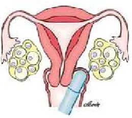
1.1.1 Oocyte retrieval
Oocytes (eggs) retrieval is the process whereby a woman's eggs are removed from
Figure 1.1 Oocyte retrieval
In order for this to occur, a woman must first have follicle (potential egg) production
stimulated by particular hormones. Once a number of follicles are produced, fertility
specialists can then remove these eggs in order to attempt fertilization.
1.1.2 Sperm collection
After the eggs retrieval, the man is asked to bring in his ejaculate in a sterile
container. The semen is allowed to liquefy at room temperature and a seminal fluid analysis
is performed (Sallam 2001). The semen is prepared for fertilization by removing inactive
cells and seminal fluid.
1.1.3 Fertilization
The eggs are then combined with the sperms in a separate dish that contains special
culture medium ready for fertilization. In normal IVF, many sperms are placed together with
an egg, in the hope that one of the sperms will enter and fertilize the egg. However, in certain
cases of severe male infertility, including such as very low sperm count or abnormally shaped
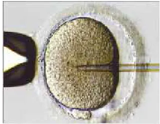
sperm or even poor sperm movement, embryologists use intracytoplasmic sperm injection
(ICSI), as shown in Figure 1.2, and take a single sperm and inject it directly into an egg. After
that the dish is then placed back inside of an incubator. As a result of fertilization, a zygote is
4
Figure 1.2 ICSI
1.1.4 Embryo cleavage
The zygote now grows to be an embryo by a cell division process and should contain:
2 cells (blastomeres): 24 hours after insemination (Day 1)
4 cells: 48 hours (Day 2)
8 cells: 72 hours (Day 3)
Morula: (Day 4)
Blastocyst: (Day 5-6)
[image:23.595.216.377.71.196.2]This development of a healthy embryo is depicted below in Figure 1.3.
1.1.5 Embryo grading
Before the implantation process, the embryos should be first examined and graded.
This examination improves success rates of pregnancies using IVF and also reduces the
number of transferred embryos which causes multifetal pregnancies. Many features have
been combined in a variety of different ways to yield different embryo scoring systems.
However, all of these scoring systems can be clustered into three main systems: zygote
scoring systems, cleaved embryos scoring systems and finally blastocysts scoring systems
(Bqczkowski et al. 2004).
Zygote scoring system
In the zygote scoring system, the evaluation is done after 16-18 hours after
fertilization and it evaluates the following features, which are shown in Figure 1.4:
• Pronuclear size and symmetry
•Size, number, equality and distribution of nucleoli
• Appearance of cytoplasm
Figure 1.4 Zygote scoring features
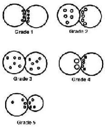
The most popular system was that introduced by Scott et al. (2000) and it has been
6
embryos and hence better results in implantations. This system uses five grades based
on both the number and distribution of nucleoli in the pronuclei, as depicted in Figure
1.5 :
Grade 1: Equal numbers of nucleoli aligned at the pronuclear junction.
The absolute number of nucleoli ranges between three and seven.
Grade 2: Equal numbers of nucleoli of equal size in the same nuclei but one
nucleus having alignment at the pronuclear junction and the other
with scattered nucleoli.
Grade 3: Equal numbers and sizes of nucleoli which are equally scattered in
the two nuclei.
Grade 4: Unequal numbers and/ or sizes of nucleoli.
[image:25.595.231.405.429.640.2]Grade 5: Pronuclei that are not aligned.
Figure 1.5 Scott's zygote scoring grades
This system was further revised and the new system classified zygotes into four
combined as Z2 zygote score while the more desirable morphologies grades such as
grades 1 and 3 were renamed Z1 and Z3.
Cleaved embryos system
In the cleaved embryos system, the evaluation is done 40-48 hours after fertilization
and it evaluates other features than that of the zygote scoring systems, simply because
the zygote was now growing to be an embryo and hence its features were changing.
These features, which are shown in Figure 1.6 include:
• Number of cells (blastomeres)
• Appearance and size of blastomeres
• Cytoplasm defects (fragments)
Figure 1.6 Cleaved embryo grading features
The Cleaved Embryo system has been adopted by many researchers including
Cummins et al. (1986), Puissant et al. (1987), Staessen et al. (1992), Steer et al.
(1992) and Zeibe et al. (1997). However, as a consequence of many research groups,
several grading techniques have been introduced, and each clinic uses its preferred
grading system. Puissant et al. (1987), for example, used the following scoring
technique:
8
Score 4:embryos with clear, regular blastomeres and either no
fragmentation or a maximum of five small fragments;
Score 3: embryos with few or no fragments but with unequal blastomeres (>
1/3 difference in size);
Score 2: embryos with more fragments but over < 1/3 of the embryonic
surface;
Score 1: fragments over > 1/3 of embryonic surface.
Two points are added if the embryo has reached the 4-cell stage by 48 h after
fertilization. This means that the maximum score of 6 points corresponds to embryos
which appear perfect and have reached the 4-cell stage 48 h after fertilization.
On the other hand, Zeibe et al. (1997) used other morphological criteria in which:
Morphology score 1.0: equally-sized symmetrical blastomeres;
Morphology score 2.0: uneven sized blastomeres;
Morphology score 2.1: embryos with 10% fragmentation;
Morphology score 2.2: embryos with 10-20% fragmentation;
Morphology score 3.0: 20–50% blastomeric fragmentation;
Morphology score 4.0: 50%blastomeric fragmentation.
Blastocysts scoring system
Finally, in the blastocysts scoring system, its evaluation is done on day 5 embryo,
when the embryo is now said to be in the blastocyst stage. The features in this stage
formation of a fluid filled cavity in the middle of the embryo (blastocoel) appears,
surrounded by a single layer of cells called trophectoderm (TE) and a small
protuberance of cells called the inner cell mass (ICM) (Zeibe et al. 1997).
Figure 1.7 Blastocyst grading features
The two most popular blastocyst embryo grading systems are the Dokras et al. (1993)
and Gardner et al. (2005) grading systems, both based on morphology. Dokras et al.
(1993) grading is based on the blastocoel's rate of development and characteristics of
the blastocoel cavity, and blastocysts are graded as BG1, BG2, or BG3. The grading
criteria used by Gardner et al. (2005) are given in Figure 1.8, and focus on blastocoel
size and developmental characteristics of the inner cell mass and trophectoderm which
are initially examined and graded from 1-6. Next, the blastocysts graded 3 through 6
are identified and their inner cell mass and trophectoderm are further graded and
10
Figure 1.8 Gardner's system (top) embryo development grading (bottom) ICM and TE grading
Despite the large number of published studies, there is no consensus about the most
accurate method for grading the embryo. The grading systems used rely mostly on factors
such as the embryologists, the IVF clinic or even religious issues. However, the work is this
Thesis considers the cleaved embryo system, which was used by the IVF clinic that provided
the work with the images.
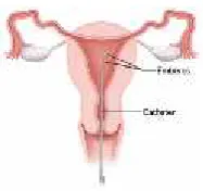
1.1.6 Transferring problem
The last stage of the IVF process is the transfer of the embryo to the woman's womb
using a catheter, as shown in Figure 1.9.
[image:29.595.251.345.622.710.2]Generally, two or more embryos are transferred during each IVF cycle. This decision
is made upon medical factors such as the number of embryos, the health of the embryos, the
patient's age and other factors such as legal issues of the fertility clinic, the country, and
sometimes religious matters. The greater the number of embryos that are transferred into the
uterus, the higher the risk of having a multiple pregnancy. When multiple pregnancies occur,
the health of both the mother and the baby can be seriously affected, so every effort to
minimize multiple pregnancies must be taken by the fertility clinics.
1.2 Problem characteristics
Since implanting more than one embryo caused multiple pregnancies, it is better for
both the mother and the baby to try to minimize the number of embryos. This requires
choosing the best embryos with the highest grades according to one of the grading techniques
mentioned before. An automated system that is able to achieve this would reduce the load on
the IVF screeners and provide a consistent and uniform selection of embryos for
implantation.
Each clinic chooses a grading system according to many issues, such as the culture
media available, the extra cost needed for longer culturing embryos and sometimes the ethical
rules of the country or even the religion. The clinic that agreed to support this work was the
Ajyal clinic in Alexandria, Egypt. This clinic re-implants the embryos on Day 2, hence uses
the Cleaved embryo grading system in particular that of Zeibe et al. (1997), and hence the
images used in this study, were Day 2, and their general appearance was the 4 cell embryo
seen in Figure 1.3 This technique examines the number of blastomeres, their size and finally
12
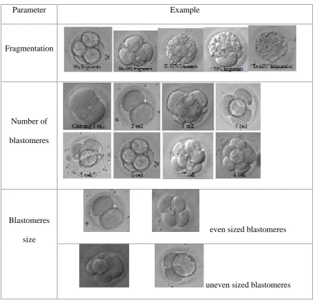
fragmentations percentages, the best of which was the first image which had 0%
fragmentation. As this percentage increases, the grading level of the embryo decreases. The
second parameter shown is the number of blastomeres. This parameter depends on the age of
the embryo, a Day 2 embryo should have 4 cells to be considered as a good embryo. As for
the last parameter, it is the size of each blastomere, they should be even sized. Therefore,
these were the features that will be used and taken into consideration upon creating the
Table 1.1 Parameters of embryo quality
Parameter Example
Fragmentation
Number of
blastomeres
Blastomeres
size
even sized blastomeres
uneven sized blastomeres
The images used in this study were taken using an inverted microscope IX71. This
microscope allows the practitioners to see and focus on the embryos. The microscope is
connected using an acquisition channel to the computer; this allows the practitioners to see
the embryos on the computer monitor using software. This software (CRONUS) is used to
capture the images used and save them in a format that allows working upon. The clinic has
14
prevented a larger number of images from being available, the images contained all possible
cases of Day 2 embryos that this work can depend upon to develop the required system. The
images have different magnification, illumination and also contain overlapping cells. These
factors are considered in designing the system. Images were divided into two datasets, one of
which contained 30 images. These were chosen to be within the same illumination brightness
and magnification and were used to develop the detection and classification algorithms. The
other 10 were used at the end to investigate the performance of the algorithms. They had
different magnifications and illumination conditions, 5 higher and 5 lower magnifications
than the 30 image training dataset. The complete dataset is shown in Appendix A (p.152).
1.3 Aims and objectives
The research question being addressed by this study is whether or not it is possible to
develop a prototype automated image analysis system that is able to detect and classify Day 2
human embryo cells as suitable for implantation. A successful system would reduce the load
on the IVF screeners and provide a consistent and uniform selection of embryos for
implantation. This will also prevent multiple pregnancies.
The specific key aims and objectives were to:
Map the characteristics and key features of the Day 2 embryo cells that would
make them suitable for implantation into features that can be detected by the
system.
Pre-process the image to compensate for magnification and illumination
variations in the microscope images.
techniques appropriate to these images.
Identify the most accurate image analysis techniques for classifying the
embryo as suitable for implantation.
Investigate the performance of the approach using images of embryos taken
with different microscope magnifications.
1.4 Thesis structure
The chapters of this Thesis are organized as follows:
Chapter 1 gives a brief introduction to the study described in this Thesis. It includes a
brief introduction to the clinical background to infertility and IVF
treatment, which leads to the importance of the grading process in
selecting suitable embryos for implantation. The dataset of microscope
images of embryos that was used is then described, followed by the aims
and objectives of the study.
Chapter 2 introduces a survey of the previous work done on the detection and
grading of embryos. This survey will include the work done on the
detection of day 1, day 2 and day 5 embryos. Finally, full analysis of the
survey will be judged and the pros and cons of each technique will be
stated.
Chapter 3 presents some of these techniques, such as image enhancement techniques,
16
Finally the software that can be used to implement such techniques will
be introduced.
Chapter 4 covers the investigation and trials of some of the common segmentation
and detection techniques on the embryos' images as a pre-processing
stage. It will also include the algorithm used to overcome the different
magnifications issue of the images.
Chapter 5 covers the implementation of the circular Hough Transform and
application to the embryo images. The technique will use some of the
pre-processing stages discussed in the previous chapter, including three
different edge-detection algorithms. The results obtained for each of
these edge-detection algorithms are compared and discussed in terms of
their robustness for cell detection.
Chapter 6 introduces a second technique that will be introduced to detect the
blastomere in the embryo. This involves template matching, with
templates being designed to match the acceptable sizes of the
blastomeres at Day 2. The template design strategy is described first,
followed by the implementation of the template matching process. Two
measures of the degree of match are investigated, and the results that
were obtained with the image dataset are presented and discussed.
Chapter 7 presents an enhanced template matching technique that was developed in
were obtained. The rationale for the enhancements, the implementation
of the new techniques and the results that were achieved when applied to
the image data set are described.
Chapter 8 gives a refinement on the binary template matching technique. This
refinement was essential to decrease the number of false cells detected
by the previous binary template matching technique.
Chapter 9 summarises all the results of the previous techniques and provides the
measure of performance of each. The technique having the best results
will be further used on the rest of the images that were left as a test
dataset. Measure will also be provided for these results.
Chapter 10 contains the summary of the work done in this thesis. It summarizes the
main aims and objectives and also summarizes the results and the
18
Literature survey
Chapter 2
Overview
This chapter introduces a survey on the previous work done on the automated analysis
of microscope images of cells in general, followed by more specific work on the detection
and grading of embryos, including Day 1, Day 2 and Day 5 embryos. Finally, the advantages
and disadvantages of these approaches and techniques are considered in the context of this
study.
2.1 Previous work on cell detection
The development of algorithms for biomedical images analysis is not an easy task, but
due to the rapid development in the bio-informatics field, much more effort has been focused
on automatic analysis of different types of cells seen through microscopes. Such cells are red
blood cells, white blood cells, tumour cell and even stem cells.
Bikhet et al. (2000) presented work that recognized and classified different categories
of normal white blood cells. The system worked on images captured by a camera attached to
the microscope and was in grey level form. Generally in blood analysis three different types
size and colour. In order to distinguish between them in terms of colour, white blood cells
appear darker in the grey-scale images than red blood cells and platelets. In the case of size,
platelets are the smallest whereas white blood cells were the largest.
The first problem that this work resolved was separating the white blood cells from
the rest of the image contents. This was achieved by first applying the median filter to the
image and then using thresholding to separate the cells from the background. After this
separation, the cells were classified into one of five different types (basophil, eosinophil,
lymphocyte, monocyte and neutrophil) according to the information about the size and
feature of each of the five types. This approach when tested on the image samples had a
percentage of correct classification of the cells of 90%. However, it did not solve the problem
of overlapping and touching cells.
Miroslaw et al. (2005) used correlation methods to detect mitotic cells automatically.
Mitotic cells are cells that have split into two cells with separate nuclei and identical
chromosomes. In this work cells were imaged using a camera attached to the microscope.
However, when viewed the cells appeared very regular and circular in shape and because of
this, the detection method was based on template matching. The templates were created either
from a 3D model or from test data. In the latter case, the templates were created by cropping
mitotic cells from test images. The 3D models differed depending on the type of the cell.
For example, for Kyoto mitotic cells, the template created for this type was a black circle
with white boundary, whereas for TDS mitotic cells, a white circle with black boundary was
used.
20
choice of the radius of the template was estimated and varied from 20 to 32 pixels and the
cell membrane was about 2 pixels thick.
The work started the detection process by applying the (3x3) median filter to suppress
any fluctuations in the intensities. Then the correlation between the image and the templates
was performed. This was followed by a peak detection stage were the highest peaks were
detected by using a suitable threshold value, but this caused the generation of many false
candidates. These were removed by the validation procedure in the last stage, which was
designed to eliminate these.
As a result of this work, it was concluded that a more sophisticated approach was
needed to cover all cases when small fluctuations in the image intensity were present. It was
also concluded that another optimisation may involve using a local threshold value instead of
using a global one, which does not take into consideration the presence of uneven
illumination.
2.2 Previous work on embryo detection
Unlike the analysis of microscope images of cells that was discussed in the previous
section which tended to be fully automated, the approaches taken by the IVF groups involved
with the detection and grading of embryo images include both automated or semi-automated
The work done by Hnida et al. (2004) determined the blastomeres' size at different
cleavage stages and defined the deviations in mean blastomere volume as a consequence of
embryonic fragmentation. The blastomere size was determined using a sequence of recorded
images of the embryos. A total of 232 embryos were used, taken after 48 hours after
fertilization, and included 2, 3, and 4 cells. However, the blastomere size of the human
embryos was analysed semi-automatically by means of morphology analysis software. This
was done using the micrometre slide with the same magnification of the embryo. A line was
drawn on the slide and since the outlined distance on the slide was known, the actual physical
distance between the two adjacent pixels was calculated. The values describing the
blastomere such as the area and the volume were then calculated automatically.
Although the aim of this work was to find a relation between the blastomere size and
the volume, rather than detect the blastomere of the embryos, the study gave several
important results. The first was that the diameter of the blastomere decreases as the number
of blastomeres in an embryo increases, and for example the mean diameter of 2-cell embryos
was 80.1 µm whereas that of 4-cell embryos was 64.9 µm, as may be seen in Table 2.1.
Table 2.1 Mean blastomere sizes of embryos at different cleavage stages (Hnida et al. (2004))
Volume
±SE (x106m3)
Diameter
±SE (µm)
2-cell embryos 0.278 ± 0.09 80.1 ± 9.8
3-cell embryos 0.182 ± 0.09 68.7 ± 12.2
22
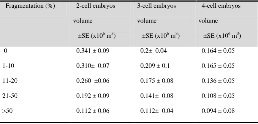
The second significant outcome was that the mean blastomere volume decreased
significantly with increasing the degree of fragmentation, indicating that the blastomere size
[image:41.595.80.515.200.409.2]could be used as an indicator of the degree of fragmentation. This is illustrated in Table 2.2.
Table 2.2 Mean blastomere volume as function of degree of fragmentation (Hnida et al. (2004))
Fragmentation (%) 2-cell embryos
volume
±SE (x106m3)
3-cell embryos
volume
±SE (x106m3)
4-cell embryos
volume
±SE (x106m3)
0 0.341 ± 0.09 0.2± 0.04 0.164 ± 0.05
1-10 0.310± 0.07 0.209 ± 0.1 0.165 ± 0.05
11-20 0.260 ±0.06 0.175 ± 0.08 0.136 ± 0.05
21-50 0.192 ± 0.09 0.141± 0.08 0.108 ± 0.05
>50 0.112 ± 0.06 0.112± 0.04 0.094 ± 0.08
Although not their main concern these researchers pointed out that computer-assisted
tools for the measuring of embryos features would be helpful.
The work described by Beuchat et al. (2008) aimed to provide a software tool that
enables the objective measuring of morphological characteristics of embryo, but for only for
the Day 1 human zygote. Their work provided measurements of new variables (24
measurements) along with the subjective ones available, as shown in Figure 2.1 on the next
page, and then showed the importance of these new measurements to the grading process. In
order to calculate these measurements, the subjective features (the pronuclei, oolemma,
cytoplasmic halo, polar bodies and finally the nucleolar precursor bodies) needed were
from a different clinic. The groups consisted of 188 images, 201 images and 107 images,
respectively.
Figure 2.1 Subjective features of human zygote
Some of these features were automatically, semi-automatically or manually detected,
as summarised in Table 2.3 .
Table 2.3 Detection method of the features
Automatic Semi-automatic Manual
oolemma yes
cytoplasmic halo yes
pronuclei yes
Nucleolar precursor bodies yes
polar bodies yes
As shown in Table 2.3, the only automatic feature detected was the oolemma of the
zygote. This was achieved by firstly detecting the foreground and the region with the central
24
belonging to the boundary of the oocyte. For this, Gaussian blur was applied followed by
Sobel edge filtering. The formed image was then binarized using Lloyd-Max classification
with two classes followed by a thinning process of the available boundary. Finally, an ellipse
fitting algorithm was fitted to this oolemma boundary.
The two features that were detected semi-automatically were the cytoplasmic halo and
the pronuclei. The detection of the cytoplasmic halo was achieved by selecting few points on
the border of the cytoplasmic halo and then applying the ellipse fitting algorithm to these
points. As for the pronuclei, a light-correction of the image was followed by histogram
equalization, then blurring with a Gaussian kernel and finally Sobel edge detection (Gonzalez
et al. 2002). After this, the edge image was correlated to edge templates and the position on
the pronuclei determined from the maximum correlated value. Finally, the nucleolar
precursor bodies and the polar bodies were manually detected because the automatic
approaches were not sufficiently robust.
Morales et al (2008) developed an automatic algorithm that helped embryologists to
have more information on the thickness of the Zona Pellucida (ZP). The purpose of this work
was to investigate the suggestion that the measurement of the ZP thickness variation was
directly related to the implantation rate. Their algorithm was based on an active contour
model, but prior to that the image had to be enhanced to increase the contrast of the image
and hence that of the ZP. The enhancement involved image thresholding followed by
applying a high-pass-Gaussian convolution filter which was optimal in terms of the
smoothing. Canny's edge detector algorithm (Canny 1986) was then applied to detect weak
edges, and then a derivative of a Gaussian filter was applied to achieve the gradient image of
was applied on the pre-processed images. When using the snake, the initial position had to be
near to the boundary of the object. This was achieved by averaging a pattern from about 60
images to determine a possible location of the centre.
The dataset used consisted of 76 images. They were taken on the second and third
days after fertilization. All images were taken using fixed magnification and brightness.
Through comparison with images manually segmented it yielded 91.65% accuracy in
localisation of the boundaries. However, this approach only detected the ZP and it did not
detect the number of blastomeres inside it.
Giusti et al. (2009) presented a practical edge-based technique for segmenting the
surrounding of the zygote cell from the rest of the image, although this did not include
detecting any of the blastomeres inside the zygote. The segmentation process was divided
into two steps. The first step found the approximate location of the cell centre, and this was
achieved by getting the image gradient followed by thresholding and then filling in the holes
of the largest component found. Hence for each point, the distance to the region boundary
was computed and the point with the maximum distance was finally chosen to be the centre.
The second step transformed the cell location to polar coordinates and the shortest-path
formulation was then used to recover the actual zygote contour. As this approach filled the
inside of the contour, it was not being able to detect the blastomeres, and so was limited to
images of Day 1 embryos.
Working on the grading of Day 5 embryos Filho et al. (2010) developed a method that
required the segmentation of the TE and the ICM, and used the segmentation features for
26
were sampled from the border. These sampled points were then used for an ellipse fitting
procedure. For the inner boundary segmentation, an initial circle situated in the centre was
used. This circle evolved until it met the inner boundary. However, this segmentation
technique did not meet the real TE boundary when manually segmented, and so, the manually
segmented approach was used to finish the calculations required for the classification. In the
case of the ICM segmentation, the circle was manually initialised at the centre of the cell and
then it evolved towards the ICM.
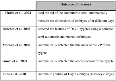
Table 2.4 summarises the relatively little work that has been done on computer-based
[image:45.595.95.500.393.676.2]analysis of images of embryos.
Table 2.4 Summary of the survey
Outcome of the work
Hnida et al. 2004 used the aid of the computer to semi-automatically
measure the dimensions of embryos after different days
Beuchat et al. 2008 detected the features of Day 1 zygotes using automatic,
semi-automatic and manual techniques
Morales et al. 2008 automatically detected the thickness of the ZP of the
zygote
Giusti et al. 2009 automatically detected the active contour of the zygote
2.3 Conclusion
After this survey of the relatively limited work that has been done on cell analysis and
the embryo detection it can be concluded that:
The first step in the segmentation and classification process was identifying
the required features of the cell and this differed from one cell to another. The
features of the red blood cells are different from those of the mitotic cells and
from many others.
The variations in the illumination, magnifications and noise in the images
required careful selection and tuning of both the pre-processing and
segmentations algorithms, but typical approaches are histogram analysis,
thresholding, applying filters and even correlation.
The analysis and classification of embryos were particularly difficult because
of the differing characteristics of embryo at Day 1, 2 and 5 and
semi-automated techniques were required in many cases.
A detected structure was considered a blastomere when the average diameter
was ≥ 40µm and a fragment when the average diameter was < 40µm. The
mean diameters of 2-, 3-, and 4- cell embryos were 80.1 ± 9.8µm, 68.6 ±
12.2µm and 64.9 ± 8.5µm, respectively.
The previous work showed the different algorithms and techniques that worked on the
segmentation of human embryos, some of which worked on Day 1, 2 or even 5 embryos, and
so provided a basis for identifying potentially effective algorithms for this study. Even so,
28
to be developed and tuned for the Day 2 images used in this study. The range of diameters of
Day 2 embryos relative to that of the ZP was identified and can be used to compensate for
magnification effects.
In the following Chapter, the basic Image Processing techniques for pre-processing
Digital Image Processing
Chapter 3
Overview
In the previous Chapter the types of image analysis techniques that have been used to
analyse microscope images of cells and support the grading of embryos were identified. This
chapter describes some of these techniques, such as those for pre-processing images, image
segmentation methodologies and object detection methods. Finally the software that can be
used to implement such techniques will be introduced.
3.1 Image representation
Digital image processing can be defined as the use of computer algorithms to
perform processing tasks on digital images. Digital images are typically represented by a
two-dimensional array M x N, where the x coordinates range from 1 to M and the y coordinates
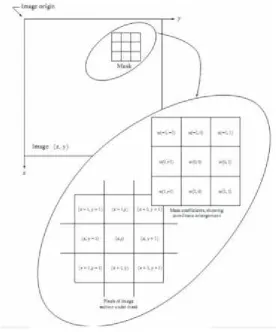
from 1 to N as depicted in Figure 3.1.
Figure 3.1 Image representation
30
The small region of the image centred on (x,y) is usually referred to as a picture
element, pixel, and has an associated value representing the average brightness in that region.
In the case of a monochrome, or grey-scale, image, each pixel value is represented by a
numeric value, which is typically in the range from 0 to 255, with 0 representing black, 255
representing white. In binary images the value of each pixel will be either 0 or 1, with 0
representing black and 1 representing white, while each pixel has a triple value in colour
images representing the contribution from the three primary colours Red, Green and Blue
colours, each value being typically in the range from 0 to 255, where 0 indicates that none of
that primary colour is present in the colour of that pixel and 255 indicates a maximum
amount of that primary colour. Since the images that we will be working on are captured by
the imaging system in grey- scale form, the following algorithms and techniques will
concentrate on grey-scale images.
3.2 Image pre-processing
The objective of the image pre-processing algorithms is to change pixel values in the
image so that it is more suitable for subsequent analysis than the original image, for a specific
application. There is no general theory of image enhancement, and the observer is the judge
of how well a particular method has worked (Gonzalez et al. 2002). The pre-processing
methods include brightness and contrast enhancement, histogram equalization, image
smoothing and filtering and are described in the following sections.
3.2.1 Image brightness and contrast enhancement
In this process the brightness of the whole image is adjusted. This involves the use of
image. An image with L grey levels has the range r= [0, L-1]. When r is the k grey level
then n is the number of pixels in the image having grey level r as seen in Figure 3.2 on
the next page.
Figure 3.2 Image histogram
Increasing or decreasing the brightness of an image is simply done by the subtraction
or addition of a constant from all pixel values. Decreasing the brightness (move the histogram
to the left) requires a subtraction operation, while increasing the brightness (move the
histogram to the right) requires an addition operation to be performed. An example of this
technique is shown in Figure 3.3 for some of the images used in this study.
Figure 3.3 Image brightness enhancement (top right) original image (top left) image after increasing the brightness (bottom) image after
32
Unlike, the brightening operations shown in Figure 3.3 which do not change the
distribution of the pixel values in the histogram, contrast enhancement is achieved by
changing the distribution of pixel values in the original image. The contrast enhancement of
the image involves scaling pixel values to stretch the histogram to cover the complete range
of grey-level values (Figure 3.4) but is does not change the general shape of the histogram
(the peak values are the same) (Awcock et al. 1995). Mathematically, the contrast adjustment
operation is defined as:
Where the input value is input and its limits are lower input and upper input and the
output value of the image after enhancement is output and its limits are lower output and
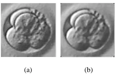
Figure 3.4 Contrast enhancement (a) original image (b) image after contrast enhancement
3.2.2 Histogram equalization
Histogram equalization is used to achieve another form of contrast enhancement. This
enhancement is done by adjusting the pixel values to produce a better distribution in the
histogram, and ideally all the histograms become equally populated. It usually increases the
global contrast of the images, especially when the -features of the image are represented by
close contrast values. However, it is also useful with the images with backgrounds and
foregrounds that are both bright or both dark.
To apply histogram equalization on a grey-scale image it is first necessary to calculate
theimage’s normalised histogram,p from:.
( ) = 0,1, … − 1
Where is the number of occurrences of grey level , L is the total number of grey
levels in the image, is the total number of pixels in the image. The contents of each
34
The cumulative distribution function is then derived from:
( ) = ( )
And finally, the transformation function, ( ) which maps each pixel value to the
new pixel value is given by:
( ) = ( − ) ∗ ( )
This procedure is illustrated in Figure 3.5. Figure 3.5(a) shows the pixels values of a
10x10 image ( =100). For simplicity, the grey levels L will be just 16, and this will make the
value of range from 0 to 15. The intermediate values in the histogram equalisation process
Figure 3.5 Example of histogram equalisation
3.2.3 Image smoothing
The aim of this process is to smooth the image in order to reduce unwanted noise and
so improve the visibility of important structures in the image. Unlike the previous techniques
where the modified value of a pixel depended only on the original value of the pixel, this
technique uses the values of the surrounding neighbourhood pixels to determine the enhanced
value of each pixel. The neighbourhood can either involve4 neighbours, as shown in Figure
36
(a) (b)
Figure 3.6 Neighbourhood (a) 4 neighbours (b) 8 neighbours
The smoothing techniques use the values of the image in the specified neighbourhood
and the corresponding values of a sub-image with the same dimensions. The sub-image is
sometimes called a filter or mask. An n x n mask means that the mask consists of n columns
and n rows, and for example, the 8 neighbour mask shown in Figure 3.6(b) is a 3x3 mask.
The process is performed by simply applying the mask from the first top left point of
the image rightwards and downwards until the end of the bottom right end of the image. At
each point (x,y), the output is given by a sum of products of each mask value and its
corresponding image pixel value. Figure 3.7 on the next page shows the 3 x 3 masking
Figure 3.7 3x3 masking process
For a mask w(x,y), with x and y having values from -1 to +1 for a 3x3 mask, the
centre of the mask, w(0,0), should coincide with the image at I(x,y) indicating that the result
R(x,y) value will replace the pixel at (x,y). The result R(x,y) is calculated using as:
( , ) = (−1, −1) ∗ I( − 1, − 1) + (−1,0) ∗ I( − 1, ) +
(−1,1) ∗ I( − 1, + 1) + (0, −1) ∗ I( , − 1) + (0,0)
∗ I( , ) + (0,1) ∗ I( , + 1) + (1, −1) ∗ I( + 1, − 1)
38 Mean (average) smoothing mask
The mean smoothing mask is shown in Figure 3.8 where it may be seen that each
element makes an equal contribution to the output.
1/9 1/9 1/9
1/9 1/9 1/9
1/9 1/9 1/9
Figure 3.8 3x3 mean smoothing mask
This masks effectively replaces each pixel value in the image with the mean
(average) value, which reduce the noise fluctuations leading to a smoother looking
image. The averaging process also reduces fine detail and makes the image look less
sharp or blurred. In Figure 3.9(a) the original image is shown and the image after
applying the mean smoothing mask is shown in Figure 3.9(b).
(a) (b)
Median smoothing
An alternative to simple averaging is median smoothing, where the pixel values of the
image coinciding with the mask are first sorted and the new pixel value is the median
(middle) pixel value. An example of this operation is shown for the 3 x 3 mask
depicted below.
The image values are 120, 126, 123, 123,150,135, 126, 125, and 145. These values are
be sorted to give: 120, 123, 123, 125, 126, 126, 135, 145 and 150. The median is the
5th element, and so the value 126 is the new value which will replace the value 150
(at the centre of the mask). Applying this mask to an image (Figure 3.10(a)), the effect
is illustrated in Figure 3.10(b).
[image:58.595.220.411.598.723.2](a) (b)
40
3.2.4 Image segmentation
The objective of the segmentation process is to partition an image into meaningful
regions which correspond to part of or the whole of objects within the scene (Awcock et al.
1995). Image segmentation algorithms are generally based on intensity discontinuity or
similarity. The first uses the abrupt changes in the pixel values which are usually associated
with the edges of an object in the image to define its boundary. The second type partitions the
image into regions that are similar according to a set of predefined criteria, such as having
values above a thresholding value. These two approaches are described in the following
Sections.
Edge detection
3.2.4.1
An edge is a set of connected pixels that lie on the boundary between two regions
(Gonzalez et al. 2002). Figure 3.11(a) shows a model of an ideal digital edge which is
available at the transition of two different grey levels intensity. However, Figure 3.11 (b) is a
practical view of the same image which shows a blurry edge rather than a sharp edge due to
many factors such as image acquisition and optical imperfection. The abrupt change in the
grey-level is shown in Figure 3.11(c) and Figure 3.11(d) shows the more realistic ramp
change in the grey-level intensity. The first derivative of Figure 3.11 (d) is given in Figure
3.11 (e). There is a positive transition at the point of going from the dark side to the lighter
side of the image; it is constant for the points in the ramp; and there is another transition at
the point from the ramp to the light side of the image. This demonstrates that the first
Figure 3.11 Different types of edges (a) ideal image (b) digital image (c) abrupt change in grey level (d) ramp change in the grey level (e) first derivative of the ramp.
The first derivative of an image is based on the 2-D gradient. The gradient G(x,y) of
an image depends on both the magnitude and orientation gradients. The magnitude gradient,
|G| , and orientation angle, α, may be calculated from :
| | = [ + ]
or
| | = | | + | |
= tan
As noise variations will appear as small discontinuities, a pixel in the image is
considered to be part of a real edge if its first derivative gradient is greater than a
pre-determined threshold value. In many cases the presence of an edge is all that is required and
so the orientation angle is not calculated.
42
Edge detection of an entire image using the magnitude gradient and orientation angle
measures can be implemented using masks with the appropriate weights. Typical of these are
the Roberts, Sobel and Prewitt edge detectors, where a pair of masks is used which are
designed to detect orthogonal components of edges, |Gx| and |Gy|, which are then combined
to give the |G| and, if necessary and the orientation angle, α.
Roberts edge detector
The Roberts edge detector uses a pair of 2x2 mask as shown in Figure 3.12. If the
pixel grey-level values in a neighbourhood are those in Figure 3.12(a), the values of
|Gx| and |Gy| are generated using the pair of masks shown in Figure 3.12(b) and
Figure 3.12(c) respectively which are sensitive to diagonal edges.
P1 P2 1 0 0 -1
P3 P4 0 -1 1 0
(a) (b) Gx (c) Gy
Figure 3.12 Roberts 2x2 masks
| | = | 1 − 4| , | | = | 3 − 2|
Sobel edge detector
The Sobel edge detector is probably the most popular basic edge detector and uses a
pair of 3x3 masks, as illustrated in Figure 3.13(b) and Figure 3.13(c) where Gx is
(a) Gx Gy
Figure 3.13 Sobel 3x3 masks
If the pixel grey-level values in a neighbourhood are those in Figure 3.13(a) then
| | = |( 3 + 2 ∗ 6 + 9) − ( 1 + 2 ∗ 4 + 7)|
| | = |( 1 + 2 ∗ 2 + 3) − ( 7 + 2 ∗ 8 + 9)|
Prewitt edge detector
The Prewitt edge detector also uses a pair of 3x3 masks but with different weights
values as illustrated in Figure 3.14(b) and Figure 3.14(c) where again Gx is sensitive
to vertical edges and Gy sensitive to horizontal edges.
P1 P2 P3 -1 0 1 1 1 1
P4 P5 P6 -1 0 1 0 0 0
P7 P8 P9 -1 0 1 -1 -1 -1
(a) (b) Gx (c) Gy
Figure 3.14 Prewitt 3x3 mask
In this case Gx and Gy are derived from:
| | = |( 3 + 6 + 9) − ( 1 + 4 + 7)|
| | = |( 7 + 8 + 9) − ( 1 + 2 + 3)|
P1 P2 P3 -1 0 1 1 2 1
P4 P5 P6 -2 0 2 0 0 0
44 Thresholding
3.2.4.2
Thresholding converts a grey-scale image into a binary image according to a pixel ‘s
grey-level value. The basic thresholding technique involves manually selecting a Threshold,
T, such that the pixels in the object(s) of interest have grey-level values greater than T, and
are set to 1 while the background is set to 0.
A refinement of this technique is to select the Threshold from a histogram of the pixel
grey-level values in the image. If the histogram has identifiable peaks and valleys as the
histogram shown in Figure 3.15, the threshold T in this case can be chosen automatically as
the valley point.