A Novel Optimised Design Using Slots for Flow Control and
High-Lift Performance of UCAVs
Usman Ali
Aeronautical Engineering
School of Computing Science and Engineering
University of Salford, Salford, UK
Submitted in Partial Fulfilment of the Requirements of the Degree of Doctor
Tables of Contents
TABLES OF CONTENTS ... II
LIST OF FIGURES ... VI
LIST OF TABLES ... XIV
ACKNOWLEDGEMENTS ... XVI
ABSTRACT ... XVII
CHAPTER 1. INTRODUCTION ... 1
CHAPTER 2. LITERATURE REVIEW ... 9
2.1. A Brief Review of Flying Wings ... 9
2.2. Aerodynamics of Flying Wing ... 12
2.2.1 Vortex Lift ... 16
2.2.2 Vortex Breakdown ... 20
2.2.3 Swept wings... 22
2.2.4 Flying Wings at Low Speed ... 26
2.3.1 Radar Cross Section ... 30
2.3.2 High Lift Devices ... 32
2.4. Role of UAVs ... 33
2.5. Computational Aerodynamics ... 36
2.6. Computational Fluid Dynamics ... 39
2.6.1 Reynolds Averaged Navier Stokes Equations ... 48
2.6.2 Turbulence Modelling ... 52
2.6.3 Near-Wall Turbulence ... 57
2.7. Vortex Lattice Method ... 61
2.8. Introduction to Optimisation ... 67
2.8.1 Optimisation Algorithms ... 68
2.8.2 Direct Search Methods ... 70
2.9. Previous Studies ... 72
2.9.1 Experimental Findings ... 73
2.9.2 Computational Findings ... 78
CHAPTER 3. RESEARCH METHODOLOGY ... 83
3.1. Experiment Methodology ... 84
3.1.1 Experiment Parameters ... 84
3.1.2 Wind Tunnel Calibration ... 86
3.1.3 Experiment Procedure... 90
3.2. Computational Methodology ... 91
3.2.1 Geometry and Grid Details ... 93
3.2.2 Boundary Conditions ... 99
3.3. Vortex Lattice Method Approach ... 107
CHAPTER 4. FLOW VISUALISATION OF CLEAN WINGS ... 111
4.1. Problem Description ... 111
4.2. Results and Discussion ... 114
CHAPTER 5. PREDICTIONS OF STABILITY AND CONTROL ... 128
5.1. Problem Description ... 128
5.2. Computational Details ... 129
5.2.1 Geometry and Grid ... 129
5.2.2 Solver Settings ... 132
5.3. Stability and Control Results ... 133
CHAPTER 6. FLOW CONTROL ... 140
6.1. Flow Control Description ... 140
6.2. Flow Control Results ... 146
CHAPTER 7. NUMERICAL OPTIMISATION ... 157
7.1. CFD Approach to Optimisation ... 157
7.2. Computational Details of Optimised Wings ... 167
7.2.1 Geometry and Mesh Details ... 168
7.2.2 Solver Settings ... 172
CHAPTER 8. CONCLUSION ... 184
REFERENCES ... 188
List of Figures
Figure 1.1: Highly swept flying wing UCAV configurations (Google, 2014) ... 3
Figure 2.1: First turbojet-powered flying wing aircraft (Okonkwo & Smith, 2016) ... 11
Figure 2.2: B2-Spirit Stealth Bomber (Okonkwo & Smith, 2016) ... 11
Figure 2.3: Four variants of delta wing planform (J.D. Anderson, 2010) ... 13
Figure 2.4: Schematic of formation of leading edge vortices over the top of a delta wing at an angle of attack (Houghton & Carpenter, 2003) ... 14
Figure 2.5: Three regions within leading edge vortex (Earnshaw, 1961) ... 14
Figure 2.6: Schematic of the spanwise pressure coefficient distribution across a delta wing (J.D. Anderson, 2010) ... 17
Figure 2.7: Lift coefficient plot for a delta wing showing an increase in lift due to leading edge vortices on the upper side of the wing (Barnard & Philpott, 2010) ... 19
Figure 2.9: The deconstruction of free stream velocity into normal and spanwise components (Barnard & Philpott, 2010) ... 23
Figure 2.10: Effects of sweepback on drag and Critical Mach number (J.D. Anderson, 2010) ... 25
Figure 2.11: Delta wing air vehicle with vertical fences on the wing (J.D. Anderson, 2010) ... 26
Figure 2.12: Classification of flow control methods (Jahanmiri, 2010) ... 28
Figure 2.13: Radar Cross Section signature at 9GHz (a) F-18E Super Hornet, (b) Northrup Grumman X-47B and (c) Generic 40° Swept UCAV (Johnston, July 2012) ... 31
Figure 2.14: Unmanned Air Vehicle Predator adapted to be used for military purposes (Barnhart, 2012) ... 34
Figure 2.15: Typical point velocity measurement in turbulent flow (Versteeg & Malalasekera, 2007) ... 50
Figure 2.16: Visualisation of turbulent flow structures (Versteeg & Malalasekera, 2007) . 50
Figure 2.17: Structure of turbulent velocity distribution near a solid wall (Bertin, 2002) .. 59
Figure 2.18: Single horseshoe vortex which is part of a vortex system on the wing (J.D. Anderson, 2010) ... 62
Figure 2.20: Nomenclature for calculating the velocity induced by a finite-length vortex
filament (Bertin, 2002) ... 65
Figure 2.21: A Graphical depiction of pattern search method (Chapra & Canale, 1985) ... 71
Figure 2.22: Cross section of a leading-edge vortex (S. A. Thompson, 1992) ... 75
Figure 2.23: Visualisation of four flow control on right side of wing. The left side of wing is uncontrolled. (a) down-stream obstacle. (b) Suction. (c) Blowing opposite the axial velocity of the vortex core. (d) Blowing along the vortex core (Mitchell & Délery, 2001)... 76
Figure 3.1: Flying wing configuration 2 mounted in low speed wind tunnel ... 85
Figure 3.2: Weight applied linearly in order to measure lift and drag ... 87
Figure 3.3: Weight linearly applied to measure pitching moments ... 87
Figure 3.4: New lift calibration with result of 0.3812... 88
Figure 3.5: New drag calibration with result of 0.0691 ... 88
Figure 3.6: New pitching moment calibration with result of -0.0103 ... 88
Figure 3.7: Aerodynamic forces and moments comparison between wind tunnel tests for configuration 1 ... 89
Figure 3.8: Typical functions in a computational aerodynamics system (Liu, 2007) ... 92
Figure 3.9: Planform view and geometric dimensions of baseline clean configuration 1 .. 95
Figure 3.11: Multi-block structured grid for clean configuration 1 ... 96
Figure 3.12: Multi-block structured grid for clean configuration 2 ... 96
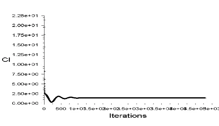
Figure 3.13: Coefficient of lift solution monitor for configuration 2 at incidence angle of 30° ... 105
Figure 3.14: Coefficient of drag solution monitor for configuration 2 at incidence angle of 30° ... 105
Figure 3.15: Moments coefficient solution monitor for configuration 2 at incidence angle of 30°... 106
Figure 3.16: VLM mesh generated in Tornado for Configuration 1 ... 108
Figure 3.17: VLM mesh generated in Tornado for Configuration 2 ... 108
Figure 4.1: Flying-wing planform geometries used for experimental and computational investigations: 40° configuration (left); and 40° with 60° cranked configuration (right) . 112
Figure 4.2: Y+ distribution on suction sides of configuration 1 (left) and configuration 2 (right) at an angle of attack of α= 30˚ ... 115
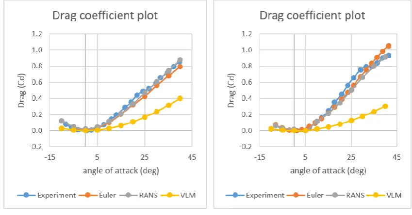
Figure 4.3: Experiment coefficient of lift comparison between configuration 1 and configuration 2 for flat plate models... 118
Figure 4.5: Lift coefficient vs angle of attack are shown: 40° configuration 1 (left) and 40° with 60° strake configuration 2 (right) ... 119
Figure 4.6: Induced-drag coefficient vs angle of attack are shown: 40° configuration (left) and 40° with 60° strake configuration (right) ... 119
Figure 4.7: Pitching-moment coefficient vs angle of attack are shown: 40° configuration (left) and 40° with 60° strake configuration (right) ... 120
Figure 4.8: Visualisation of the vortex system on the upper surface of configuration 2 for incidence angles from α = 5° to α = 20° ... 123
Figure 4.9: Mach number distribution on the upper surface of configuration 2 for incidence angles from α = 5° to α = 20° ... 124
Figure 4.10: Absolute helicity based Iso surface for incidence angles of α = 20° to α = 40° ... 124
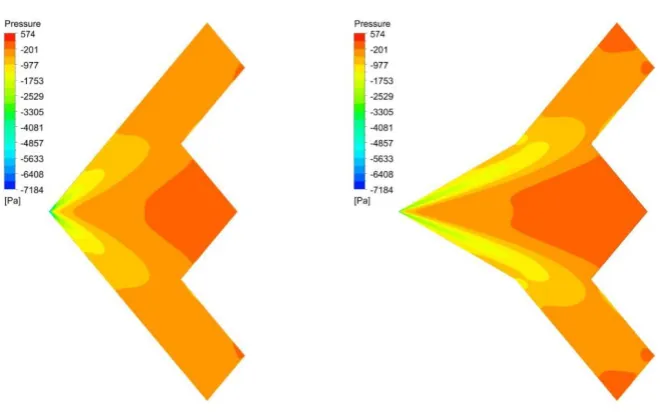
Figure 4.11: Plots of pressure coefficient distribution and wall shear vectors at incidence angles of α = 15° and α = 20° ... 125
Figure 4.12: Pressure distribution and surface streamlines on upper surface of configuration 2 for incidence angles from α = 5° to α = 20° ... 125
Figure 5.1: Trailing edge control surface deflected up at an angle of 10° on configuration 1 ... 130
Figure 5.3: Aerodynamic coefficients and moments comparison between clean and control surface models with respect to angle of attack ... 135
Figure 5.4: Aerodynamic forces and moments for configuration 1 in sideslip angle of 30° ... 137
Figure 5.5: Pressure distribution and skin friction lines for alpha = 10° and beta = 30° (left); alpha = 20° and beta = 30° (right)... 137
Figure 6.1: Dimensions of leading-edge slot on highly swept flying wing called configuration 2 in this study ... 141
Figure 6.2: Dimensions of chordwise slot on highly swept flying wing called configuration 2 in this study ... 142
Figure 6.3: Meshed configuration 2 with leading-edge slot (left); chordwise slot (right) 142
Figure 6.4: Wings used for the calculations of coefficients of lift ... 145
Figure 6.5: Topology of unstructured grid used for highly swept wing ... 145
Figure 6.6: Comparison of aerodynamic coefficients and pitching moments between clean and leading-edge slot models... 148
Figure 6.7: Pressure distribution and surface streamlines comparison between clean and leading-edge slot models at incidence angle of 5° ... 151
Figure 6.9: Pressure distribution and surface streamlines comparison between clean and
chordwise slot models at incidence angle of 25° ... 152
Figure 6.10: Lift difference comparison between wings with and without chordwise slot at constant angle of attack of 20° ... 154
Figure 6.11: Lift difference comparison between wings with and without chordwise slots at constant control deflection of 5° ... 155
Figure 7.1: Positions of chordwise slot for the optimisation analysis, Locations 1 - 8 ... 161
Figure 7.2: Widths of chordwise slot for the optimisation analysis, 0.5mm - 2mm ... 161
Figure 7.3: Lengths of chordwise slot for the optimisation analysis, 0.06m - 0.10m ... 162
Figure 7.4: Angles of chordwise slot with respect to trailing edge for the optimisation analysis, 130° - 60° ... 162
Figure 7.5: Dimensions of optimised chordwise slot ... 163
Figure 7.6: Horizontal lines on the trailing edge of chordwise slot wing that were used to calculate mass flow rate of the wing ... 163
Figure 7.7: Mass flow rate as a function of location with interpolated data ... 164
Figure 7.8: Mass flow rate as a function of location with interpolated data ... 164
Figure 7.9: Mass flow rate as a function of length with interpolated data ... 165
Figure 7.11: Flying wing configurations with optimised chordwise slot: Flat plate model
(left); GOE444 aerofoil profile wing (right) ... 169
Figure 7.12: Y+ values for optimised flat plate slot wing at incidence angle of 30° ... 170
Figure 7.13: Y+ values for optimised GOE444 slot wing at incidence angle of 30° ... 171
Figure 7.14: Topology of unstructured grid for GOE444 wing ... 171
Figure 7.15: Convergence monitors for optimisation analysis: Residual convergence (left); Lift, Drag and Moments (right) ... 173
Figure 7.16: Horizontal lines along trailing edge on top and bottom surfaces of the model ... 175
Figure 7.17: Mass flow rate comparison between clean and chordwise cavity flat plate wings ... 175
Figure 7.18: Aerodynamic coefficients and moments comparison between clean and optimised chordwise cavity flat plate wings ... 176
Figure 7.19: Aerodynamic coefficients and moments comparison between clean and chordwise cavity for flat plate, GOE444 and NACA0008 configurations ... 180
Figure 7.20: Mass flow rate comparison between clean and chordwise cavity models for GOE444 aerofoil sections ... 181
List of Tables
Table 2.1: Number of transport equations solved for RANS turbulence models ... 53
Table 3.1: Reference values for the wind tunnel models ... 86
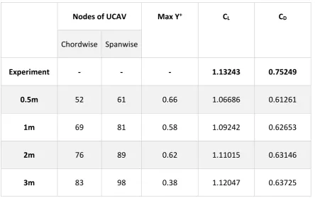
Table 3.2: Comparing grid refinement results for configuration 1 at incidence angle of 19.2° ... 97
Table 3.3: Comparing grid refinement results for configuration 2 at incidence angle of 29° ... 97
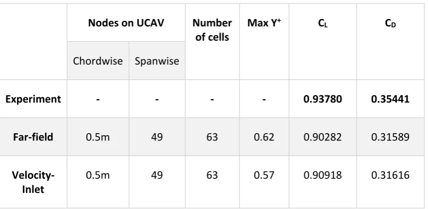
Table 3.4: Comparison of compressible and incompressible computations wherein solutions for far-field and velocity-inlet boundary conditions are analysed for configuration 1 ... 101
Table 3.5: Comparison of far-field boundaries placed at 10c and 15c from the wing for configuration 2 ... 101
Table 4.1: Reference values for CFD computations ... 115
Table 6.1: Number of elements used for clean, leading-edge and chordwise slot wings for flow control investigations ... 143
Table 6.2: Number of elements used for the computations of wings ... 146
Acknowledgements
Abstract
In this study, two UCAV planforms are considered based around generic 40° edge-aligned configurations. One configuration has a moderate leading and trailing edges sweep of Λ = 40°, while the other configuration is highly swept with a leading-edge sweep of Λ = 60° and trailing edges sweep of Λ = 40°. The objectives of the present study on UCAV configurations are two-fold: first to predict aerodynamic performance particularly the maximum-lift characteristics of two flying wing planforms; second to control the flow by inserting leading-edge and chordwise slots and analysing the viscous flow development over the outboard sections of a flying-wing configuration to maximise the performance of control surfaces.
The first part is demonstrated using a variety of inviscid Vortex Lattice Method (VLM) and Euler, and viscous CFD Reynolds Averaged Navier-Stokes (RANS) methods. The computational results are validated against experiment measured in a wind tunnel. The VLM predicts a linear variation of lift and pitching moment with incidence angle, and substantially under-predicts the induced drag. Results obtained from RANS and Euler agree well with experiment.
Chapter 1.
Introduction
that although leading-edge slots have been used on low sweep wings to enhance the lift of
air vehicles, to the best of the author’s knowledge they have not been used to maximise the performance of control surfaces on highly swept flying wing configurations. Furthermore, the author has not found any literature on flying wing configurations where chordwise slots have been used for the purpose of passive flow control. Therefore, this is novel strand of the research.
a) Northrop Grumman B-2 (Barnard & Philpott, 2010)
b) BAE Systems Taranis (Lee, 2016)
c) Future UCAV Concept (Gursul, Gordnier, & Visbal, 2005)
d) Boeing X-45A (Cummings, Morton, & Siegel, 2008)
These swept wing vehicles have desirable characteristics of low drag at high speeds. Moreover, they continue to produce lift up to high angles of attack by taking advantage of the additional lift generated by the leading-edge vortices. Leading edge vortex is the main element of flow over swept wings, as it provides lift for flight control at high angles of attack (J.D. Anderson, 2010); (Houghton & Carpenter, 2003); (Wilson & Lovell, 1947); (Hummel & Srinivasan, 1967). A disadvantage, however, is that as the angle of attack is increased, the leading-edge vortices become detached and experience a forward migration or lateral flow to the outboard sections of the wing. The intensity of this forward migration of flow to the outer panels of the vehicle grows in intensity with higher angles of attack (Frink et al., 2012); (Kerstin et al., 2012); (Barnard & Philpott, 2010). As a result of this forward migration of flow to the outer panels of the vehicle, the roll control contributed by trailing edge control surfaces becomes severely restricted, as control surfaces would be operating in a separated flow (Gudmundsson, 2014a); (Barnard & Philpott, 2010); (Shevell, 1989). Therefore, high lift generated by leading-edge vortices cannot be exploited, as control surfaces become ineffective in producing the control forces required for the lateral control of air vehicle at medium to high angles of attack. In addition to the deterioration in roll stability, a powerful nose pitch-up moment is experienced by air vehicle as angle of attack approaches stall (Gudmundsson, 2014a); (Kermode, 2012).
detrimental effects on RCS signature, hence they must be avoided (Schütte et al., 2012); (Barnard & Philpott, 2010). Therefore, as an alternative to the above methods, leading-edge and cross-flow slots are used for the first time on a flying-wing configuration and they successfully control the flow by maximising the lift over control surfaces at medium to high angles of attack. With smooth and higher airflow rate over the control surfaces, good roll control can be retained by the air vehicle at medium to high angles of attack (Shevell, 1989). It should be noted that the slots under study lie flush with the surface of the wing, and as a result the effect on RCS signature is expected to be minimal when compared to standard flow-control techniques.
There are two main aims of this study. The first is to enhance our understanding of the flowfield over two low observable UCAV configurations, and their prediction of high-lift performance using high and low fidelity CFD techniques. High-lift performance of an air vehicle can have major influence on vehicle’s weight and stability. Therefore, accurate
predictions of high-lift performance are of paramount importance. The second aim is to determine whether chordwise slots in the wing improved the lift coefficient at high angles of attack upon control surface deflection and to control lateral flow development on the upper surface of the wing using leading-edge and chordwise slots, and to develop a novel optimised design using a slot to maximise the performance of control surfaces at moderate to high angles of attack.
stabilities were assessed and the flow features responsible for nonlinearities were highlighted. Computational studies were performed to understand the capabilities of inviscid and viscous flow methods to predict the high lift characteristics, and to analyse the viscous flow development over the outboard sections of UCAV configurations. The flowfield on the upper surface of swept wings was visualised with streamlines. Grid refinement investigations were carried out to examine the effects of grid resolution on the solution. Moreover, computational investigations into turbulence models, boundary conditions, and solvers were performed to analyse the effect of different computational choices on the solution of flying wing configurations.
The second aim was achieved by performing computational investigations for flow control on wings with leading-edge and chordwise slots. The results of computational investigations were compared with clean configurations and verified with experiment. Leading-edge and chordwise slots were considered because they lie flush with the surface of the wing, and thus are expected to have a reduced RCS signature. A novel optimised design was developed for a chordwise slot using a numerical optimisation method. The optimised design was implemented on a highly-swept UCAV configuration to maximise the performance of trailing edge control surfaces of the wing. The mass flow rate normal to trailing edge of optimised UCAV configuration was measured and compared with the clean configuration.
Chapter 2.
Literature Review
2.1.
A Brief Review of Flying Wings
speeds, resulting in a fuel-efficient aircraft design. Therefore, flying wing systems emit less pollutants as they burn less fuel, making it more environmental friendly (Okonkwo & Smith, 2016). The flying wing system also has low noise signature when compared with conventional air vehicles (Mistry, 2009); (Kundu, 2014).
The concept of a flying wing aircraft was introduced by a German Engineer Dr. Adolph Busemann at Fifth Volta Conference held in Rome in September 1930. Although, Dr. Busemann is credited with introducing the concept of a flying wing, but another German Engineer, Dr. Alexander Lippisch, had been experimenting with swept wing and tailless aircraft for several years, and he is credited with the first flight of a swept wing aircraft in 1931. Dr. Lippisch was primarily interested in reducing the aerodynamic drag and increasing the flight speeds, therefore he chose to explore the potentials of a flying wing design (Pattillo, 2001); (S. A. Thompson, 1992). The desire to increase flight speeds was found in many parts of the aviation industry at that time, but the concept of a flying wing was not investigated to its full potential until the development of jet engine in the early
1940’s. After the introduction of jet engine in aviation, transonic speeds became
attainable, and therefore research investigations on swept wing aircrafts soon began to increase (S. A. Thompson, 1992); (Pattillo, 2001).
Figure 2.1: First turbojet-powered flying wing aircraft (Okonkwo & Smith, 2016)
Jack Northrop in United States explored the potentials of flying wing concept, as he was convinced of aerodynamic advantages of wing sweep and fewer control surfaces on an air
vehicle. Northrop established the Northrop’s corporation in 1927, building several flying
wing aircrafts including N-1M, N-9M, XB-35, YB-35 and so on (Okonkwo & Smith, 2016).
The most successful flying wing aircraft of Northrop Corporation was developed in 1980s, after the advent of modern fly-by-wire technology. The aircraft in question is known as B2 Spirit, and is shown in Figure 2.2. The primary advantages of B2 bomber include stealth design, better payload carrying capability and considerably better flight control characteristics due to the incorporation of fly-by-wire technology (Okonkwo & Smith, 2016); (Rehman, 2009). Some of the earliest contributions to the Flying Wing design were also made by Lt. John Dunne in United Kingdom. Dunne realised the importance of wing sweep and incorporated it in his tailless glider and series of powered bi-planes (Rehman, 2009).
2.2.
Aerodynamics of Flying Wing
2007). When the capability of a flying wing aircraft at medium to high angles of attack is taken into consideration, the presence of leading-edge vortices must be considered. The understanding of leading-edge vortices can be furthered by examining the flowfield of delta wings shown in Figure 2.4.
Figure 2.4: Schematic of formation of leading edge vortices over the top of a delta wing at an angle of attack (Houghton & Carpenter, 2003)
Experimental investigations have established that at relatively low angles of attack the flow separates from the leading edges and rolls into two vortex sheets of rotating fluid (Lambourne & Bryer, 1959); (Earnshaw, 1961); (Delery, 2001); (Elle & Britain, 1961) as illustrated in Figure 2.4. When sharp leading edge of the wing is encountered, a free shear layer is formed which rolls into a vortex. This phenomenon transpires on both sides of the wing, resulting in the formation of two counter rotating vortices. This pair of vortices is the cause of high lift and delay in wing stall to a higher angle of attack for delta wing configurations (J.D. Anderson, 2010). The angle of attack at which these vortices are first formed is mainly a function of wing sweep angle (Gursul, Wang, & Vardaki, 2007), as will be explained in a later section.
As noted earlier, the separated vortex flows under the influence of vorticity contained within it, rolls up in a spiral fashion to form a primary vortex pair (Wilson & Lovell, 1947); (Lambourne & Bryer, 1959) shown in Figure 2.4. The inner core region in the centre of the vortex is influenced by the viscous forces as illustrated in Figure 2.5, and has characteristics of large velocity and pressure gradients. The core gives rise to strong swirling velocities and associated with this a strong negative pressure on the suction side of the wing (Earnshaw, 1961); (J.D. Anderson, 2010). The primary vortex pair creates lateral boundary layer on the suction side of the wing, colliding with the primary separation and resulting in secondary vortex as shown in Figure 2.4. The secondary vortex is smaller and weaker, is located outboard and rotates in opposite direction to the primary vortex. However, unlike primary vortex, strength and size of secondary vortex is dependent on Reynolds number, and is a function of area covered by the lateral boundary layer flow. This system of vortical flows exist up to very high incidence angles for delta wing planforms (Delery, 2001); (Frink et al., 2012).
2.2.1 Vortex Lift
leading edge vortices on the upper side of the wing (Polhamus, 1969); (Campbell & Osborn, 1986); (Newsome & Thomas, 1986).
They leading edge vortices formed on both sides of delta wing are strong and stable, and consequently they increase the energy of vortex flows. This results in local static pressure to drop in the vicinity of leading-edge vortices. Therefore, surface pressure on the upper side of wing is reduced near the edges of the delta wing, but remains reasonably constant over the middle of the wing as is shown in Figure 2.6. It should be noted that Figure 2.6 shows the spanwise pressure variation over the upper surface of a delta wing (J.D. Anderson, 2010).
Figure 2.6: Schematic of the spanwise pressure coefficient distribution across a delta wing (J.D. Anderson, 2010)
remains constant in the mid-section but lower than the freestream pressure. The considerable drop in pressure over the upper surface can be observed near the edges of delta wing, depicted by vertical arrows in Figure 2.6. This is the result of leading-edge vortices creating a strong suction over the top surface of the wing near the edges of the delta wing. The length of arrows in Figure 2.6 represent the local lift contribution of each section on the upper and lower sides of the delta wing (J.D. Anderson, 2010).
This suction effect is the cause of lift enhancement over delta wings, and the reason why delta wing configurations obtain much higher lift coefficients for angles of attack at which conventional wings would normally stall (J.D. Anderson, 2010). The separated vortices on the upper surface of the wing make an extra contribution to lift known as vortex-lift (Polhamus, 1969); (Barnard & Philpott, 2010). For subsonic flows, total lift of delta wings is a combination of attached potential flow and vortex lift. This method is termed as the leading-edge suction analogy and can be represented by the following equation:
𝐶𝐿 = 𝐾𝑃𝑠𝑖𝑛𝛼𝑐𝑜𝑠2𝛼 + 𝐾
𝑉𝑐𝑜𝑠𝛼𝑠𝑖𝑛2𝛼 (2.1)
Figure 2.7: Lift coefficient plot for a delta wing showing an increase in lift due to leading edge vortices on the upper side of the wing (Barnard & Philpott, 2010)
2.2.2 Vortex Breakdown
At high angles of attack, leading edge vortices undergo a transition known as vortex breakdown or vortex bursting shown in Figure 2.8. The phenomenon of vortex breakdown was first observed in a water tunnel, where it was discovered that vortex flow undergoes an abrupt decrease in the magnitude of axial and circumferential velocity components (Peckham, 1958), and core of the vortex suddenly increases in cross sectional area when incidence angle is increased beyond a critical angle of attack. It can be observed from Figure 2.8 that upstream of vortex breakdown, the flow is tightly bound, but downstream of vortex breakdown the flow is highly turbulent. The vortex breakdown causes the flow to become stagnant, exhibiting large scale of unsteadiness (Lambourne & Bryer, 1961).
Figure 2.8: Water tunnel visualisation of vortex breakdown over a delta wing at an angle of attack (Cummings, Forsythe, Morton, & Squires, 2003)
2.2.3 Swept wings
With the advent of jet engine transonic speeds became possible, and research started to focus on problem of raising the critical Mach number by delaying the onset of shockwaves (Kermode, 2012). It is a formidable task to design a wing that behaves well in both low and high speed flows, as flows of different types can drastically change the control and stability characteristics of air vehicle (Barnard & Philpott, 2010). Wing sweep is often used on both civil and military aircrafts to reduce the effects of compressibility at transonic speeds. It should be noted that wing sweep can be backward sweep or forward sweep. The latter type of sweep is less common and is not considered in this study. The purpose of the wing sweep is twofold: first to raise the critical Mach number of flows by delaying the onset of shockwaves; and second to resolve a potential Centre of Gravity (CG) problem in an aircraft design (Gudmundsson, 2014a). In a low speed aircraft, wing sweep allows to fix Centre of Gravity (CG) problem if it is discovered that CG is further forward or aft than expected. Backward wing sweep was used for this purpose on DC-3 Dakota, and forward sweep was used on SAAB MFI-15 Safari to solve the CG issue that resulted from the engine and two occupants sitting in front of the main spar (Gudmundsson, 2014a).
increase in nose-down pitching moment in a phenomenon termed as Mach-tuck (Gudmundsson, 2014a).
The Figure 2.9 illustrates how wing sweep raises the critical Mach number and delays the onset of shockwaves. The airflow can be divided into two components of velocity, one normal to the span and one along the direction of the span of the wing. The component of velocity along or parallel to the span can be ignored as it does not change considerably as the flow passes over the wing. The normal component of the velocity is responsible for the pressure distribution but it is lower than the freestream velocity (Barnard & Philpott, 2010); (Kermode, 2012). The normal component can be represented by the free stream velocity 𝑉∞, and leading-edge sweep angle 𝛹 by the following relationship:
𝑉𝑛 = 𝑉∞𝑐𝑜𝑠𝛹 (2.2)
With sufficient wing sweep, the normal component of the velocity becomes considerably slower than speed of the sound even when aircraft is flying in supersonic speed regimes (Kermode, 2012); (Barnard & Philpott, 2010). A look into flow past a section of a swept wing reveals that flow patterns and general flow features are similar to ordinary subsonic flow as long as normal component of the velocity remains subsonic. Even when resultant of normal and spanwise components of velocity has become supersonic in places, the flow features remain subsonic.
The wings of aircraft have to be swept even when aircraft is not intended to fly at supersonic speeds, as airflow becomes supersonic on the upper surface of the wing where it is moving faster than the freestream velocity. This phenomenon occurs when aircraft has a flight speed of 60 to 70 percent of the speed of the sound. Civil aircrafts for medium to long-haul flights fly faster than 70 percent of the speed of the sound, therefore swept wings are used to delay the onset of shockwaves on such aircrafts (Barnard & Philpott, 2010).
their advantages when aircraft is designed to cruise close to or above speed of sound. However, sweep should be avoided on a low speed aircraft unless necessary (Barnard & Philpott, 2010); (Gudmundsson, 2014a).
Figure 2.10: Effects of sweepback on drag and Critical Mach number (J.D. Anderson, 2010)
introducing a washout in the wing design (Coppin, 2014). The washout prevents tip stalling first by keeping root at higher angle of attack than the tip of the wing when aircraft approaches stall (Kermode, 2012); (Barnard & Philpott, 2010).
2.2.4 Flying Wings at Low Speed
The idea behind wing sweep is that by putting the leading edge at an angle relative to the direction of air flow, the critical Mach number can be delayed. This results in reduced wave drag, making air vehicles under consideration suitable for high cruise speeds (Gudmundsson, 2014a); (Barnard & Philpott, 2010); (S. A. Thompson, 1992). However high speed air vehicles, such as one shown in Figure 2.11, fly at low speeds for take-off and landing, and spend most of their time flying at subsonic speeds using supersonic capability only for short periods of time (J.D. Anderson, 2010).
At subsonic speeds, the aerodynamic behaviour of swept wing vehicles is different than the high aspect ratio wings (Gudmundsson, 2014a). The performance of swept wing vehicles at low speeds is crucial as the mission roles of modern air vehicles require them to operate at low speed and variety of alpha conditions during various flight phases such as take-off and landing (Houghton & Carpenter, 2003); (J.D. Anderson, 2010). Therefore, understanding of aerodynamic properties of subsonic flows for these vehicles is essential.
As noted earlier, one of the unique aspects of flying wing configurations is that they generate high lift at high angles of attack. This aspect of flying wings makes them suitable for military applications, as such applications have begun to encompass very high incidence angles for their flight envelopes (Robert et al., 2007). Furthermore, flight operations such as landing, take off and combat manoeuvring are encountered at moderate to high angles of attack regimes (Coppin, 2014). Therefore, flow physics of subsonic flows for flying wing configurations at moderate to high incidence angles is of immense significance. It should be noted that the high lift generated by the leading edge vortices on delta wing configurations cannot be fully exploited due to the spanwise flow to the outboard sections of the wing (Shevell, 1989); (Coppin, 2014). One of the objectives of this research is to control the spanwise flow on the outboard sections of the wing to enhance the lateral control of the flying wing configurations.
2.3.
Introduction to Flow Control
This study explores the flow control mechanisms which can limit the development of the lateral flow to the outboard sections of a flying wing configuration. The objective is to route more airflow over the control surfaces of the trailing edges of the air vehicle. More airflow over the control surfaces will result in effective lateral control of air vehicle at medium to high angle of attack (Barnard & Philpott, 2010); (Shevell, 1989).
Figure 2.12: Classification of flow control methods (Jahanmiri, 2010)
review and analysis on active flow control has been provided by Jahanmiri (Jahanmiri, 2010).
Active flow control requires some form of energy input in order to manipulate the flow structures over the wing. Active flow control schemes are further divided into predetermined and interactive methods. Predetermined control loops refer to steady or unsteady energy inputs without consideration for the state of the flowfield, and thus sensors are not required for this method. In reactive scheme, sensors are used continuously to adjust the controller or energy input. The control loop for interactive scheme can either be feed forward (open) or feedback (closed) loop as shown in Figure 2.12. In feed forward loop, the sensors are placed upstream of the controller (Jahanmiri, 2010). In past active flow control concepts of various types have been used that can successfully improve the aerodynamic characteristics of air vehicles. Efforts to control the structure and trajectory of leading edge vortices on swept flying wings, using active flow control approaches, have included suction and blowing at the leading edges (Joslin, Miller, & Lu, 2000). Active flow control methods to control the leading-edge vortices and vortex break breakdown for improved aerodynamics of swept wing vehicles have been described by Gursul (Gursul et al., 2007) and Nathan (Nathan, Zhijin, & Ismet, 2008).
Anderson, 2010); (Gudmundsson, 2014b). In present study, however, it is not feasible to add such control surfaces due to their adverse effect on Radar Cross Section (RCS) signature of flying wing configurations. As a result, novel flow control mechanisms must be investigated in order to manipulate the flowfield structures over flying wing without leading to the loss of control of the air vehicle. The challenge is to achieve that change with a simple device that is inexpensive to build and operate, and has minimum side effects with respect to RCS signature.
2.3.1 Radar Cross Section
Radio detection and ranging commonly known as Radar, transmits radio waves to detect the presence of an aircraft and find its position. The principle of the radar is that a transmitter sends out radio signals which are reflected back to the source or a receiver when an object is encountered (Kingsley & Quegan, 1992). When transmitter and receiver are located on same platform and share the antenna, the radar is called monostatic. The radar is referred as bistatic, when radar transmitter and receiver are at two different locations.
energy away from the source into the space. The planform alignment or shaping of a stealth aircraft is generally considered to be most important line of RCS control (Bertin, 2002); (Coppin, 2014). The shaping of aerial vehicles under discussion leads to unconventional planform shapes that are associated with the term stealth. As noted earlier, the stealth designs are aerodynamically unstable, as vertical tails and conventional control surfaces are absent from these aerial vehicles (Schütte et al., 2012). For the aircraft with curved or perpendicular surfaces, the returns to the source will be strong (Coppin, 2014). An example of this phenomena is shown in Figure 2.13 where a conventional fighter aircraft is compared with two stealth UCAVs.
Figure 2.13: Radar Cross Section signature at 9GHz (a) F-18E Super Hornet, (b) Northrup Grumman X-47B and (c) Generic 40° Swept UCAV (Johnston, July 2012)
2.3.2 High Lift Devices
Devices or modifications to the wing that increase maximum lift coefficient and stall angle of the aerofoil are called high lift devices (J.D. Anderson, 2010). Air vehicles use various high lift devices to increase landing and take-off performance of the aircraft. High lift devices allow the air vehicle to operate at stall speeds during landing and take-off, resulting in shorter runway requirements. The stall speed of air vehicle is the lowest speed at which controllable flight can be sustained (Shevell, 1989); (Gudmundsson, 2014b). Therefore, objective is to reduce stall speed as much as possible when designing a wing. This can be achieved by increasing the camber of the wing and delaying flow separation by adding energy to the boundary layer (Bertin, 2002); (Moran, 2012); (Rathakrishnan, 2013) (Schlichting, Gersten, Krause, Oertel, & Mayes, 1960).
slot is therefore highly dependent on the geometry of the wing and the leading-edge device mounted on the wing (Gudmundsson, 2014b).
Trailing edge high-lift device increases the maximum lift coefficient of wing by increasing the camber, but this usually results in reduction of stall angle as well (Kermode, 2012); (Gudmundsson, 2014b). Some of the common trailing edge flaps include plain flap, split flap, external flap, single-slotted flap, double-slotted flap, fowler flap and Gurney flap. The performance of these trailing edge devices has been comprehensively reviewed by Gudmundsson (Gudmundsson, 2014b). In this study, trailing edge flaps were mounted and computationally analysed on a moderately swept flying wing configuration and comparison was made with a clean model in Chapter 5 of the thesis. Flying wings do not use horizontal stabiliser, and therefore combine the functions of elevators and ailerons into one set of flight control. For a flying wing, control surfaces on the trailing edge of the wing deflect up or down at the same time like an elevator to provide pitch control, and they are also able to move in an opposite direction to each other like ailerons to give roll control to a flying wing (J.D. Anderson, 2010).
2.4.
Role of UAVs
autopilot in case of emergencies (Barnhart, 2012). The amount of system autonomy has huge effect on UAV development though, as project becomes more complex and expensive with increased autonomy of the air vehicle (Clark, 2000). It should be noted that UAVs under consideration in this study are designed to be returned and reused, and they do not have a human on board. The generic terms drone, remotely piloted vehicle (RPV) or remotely piloted aircraft (RPA) are sometimes used interchangeably for UAVs under discussion (Clark, 2000); (Barnhart, 2012).
Figure 2.14: Unmanned Air Vehicle Predator adapted to be used for military purposes (Barnhart, 2012)
be deployed in a high-risk environment without the need to risk a pilot’s life. They are more cost effective in comparison to manned aircraft, as pilot and associated life support system is not required to operate such air vehicles (Clark, 2000). Moreover, they can perform manoeuvres that human pilots will not be able to withstand (Kermode, 2012).
Some UAVs such as Predator can be adapted for offensive use by fitting them with air-to-surface missile. The Predator, shown in Figure 2.14, was originally designed to carry out intelligence gathering, surveillance, and reconnaissance or ISR missions, but in recent years it has been adapted to deliver hellfire missiles on enemy targets (Barnard & Philpott, 2010); (Barnhart, 2012). Civilian applications of UAVs not only include surveillance but they are also being used for mapping, traffic monitoring, land resource management and so on (Barnard & Philpott, 2010).
such as Boeing X-45A, Northrop Grumman X-47B, BAE Systems Taranis (Barnhart, 2012). Some of the roles of modern UCAVs include flying surveillance missions, strike and suppression of enemy defences, bomb damage assessment and so on (Clark, 2000).
Aviation technology has made great leaps in mechanics, structures, materials, and power delivery in last 20 years (Barnhart, 2012). UCAV research has benefited from these advancements but technical and aerodynamic challenges associated with low observable air vehicles remain considerable (Lee, 2014); (Clark, 2000). The integration of mature technologies into UCAV operational system, and making close-hand technologies affordable are two great challenges in the developments of future UCAVs (Clark, 2000).
The UCAV market is anticipated to experience strong growth in the coming years. A team of market research analysts, Teal Group Corporation, has predicted that UAV sector of aerospace is going to be most dominant sector in terms of growth, with expenditures expected to grow substantially (Barnhart, 2012).
2.5.
Computational Aerodynamics
and also establish the validity of experimental data. Numerical computations provide a new dimension in the analysis and solution of aerodynamic problems, and moreover they are more cost effective than laboratory experiments. One of the early achievements of
Computational Aerodynamic methods was with NASA’s aircraft called HiMAT. Wind tunnel
tests had established that HiMAT would have unacceptable drag levels at speeds of Mach 1. If NASA had redesigned HiMAT using wind tunnels, the cost would have amounted to $150,000, and additionally it would have delayed the project. The wings of aircraft were redesigned using a computer program at the cost of $6000, saving NASA substantial amount of money and time (John D. Anderson, 1995).
The process of aircraft design can be aided using numerical methods by focusing on smaller elements of aircraft such as flow over an aerofoil with a control surface, and internal flows such as compressors, burners, turbine blades and so on. The usefulness of such flows is that it can show flow imperfections in a localised region, which can then be rectified by modifying the design. The amount of wind tunnel testing for the development of novel designs has been greatly reduced with the advent of computational aerodynamics, as computer programs can be used to test design options and parameters of aircrafts (Pozrikidis, 2017); (Cummings, 2015).
divided into linear and non-linear methods. Linear methods are less computer intensive, and they require a solution of large system of linear equations that would be too laborious to solve otherwise (Moran, 2012). Panel Method and Vortex Lattice Method are two widely known linear techniques for aeronautical applications.
As computer processing speeds and memory became faster and bigger, engineers soon began to solve more difficult non-linear problems in fluid dynamics. This gave rise to whole new discipline – Computational Fluid Dynamics (CFD), which has become a leading method in the prediction and solution of aerodynamic problems (Cummings, 2015). The major target of CFD process is to enhance design process of any problem that deals with fluid flow, therefore CFD codes are structured around the numerical algorithms that can solve all kind of fluid flow problems not just aerodynamic problems (Pozrikidis, 2017). Today CFD has found its applications in range of Engineering disciplines including automobile and engine, industrial manufacturing, civil engineering, environmental engineering, naval architecture and so on (John D. Anderson, 1995).
computational time and cost for the resolution of aerodynamic problems. In this study, Vortex Lattice Method (VLM), Euler and RANS approaches were used to analyse and validate the experimental data of clean and cavity wings.
2.6.
Computational Fluid Dynamics
All of the fluid dynamics is based upon fundamental governing principles of continuity, momentum and energy equations (Versteeg & Malalasekera, 2007). These physical principles can be described as: a) Principle of conservation of mass i.e. the mass of fluid is conserved; b) The rate of change of momentum equals the sum of the forces on a material element (Newton’s second law); c) Principle of conservation of Energy i.e. energy is conserved (the first law of thermodynamics) (Versteeg & Malalasekera, 2007). The physical principles under discussion represent mathematical statements of conservation laws and can be written as follows (John D. Anderson, 1995):
Continuity Equation
𝜕𝜌
𝜕𝑡 + ∇ ∙ (𝜌𝑉) = 0
(2.3)
In Cartesian coordinates, the vector operator ∇ is described as
∇≡ 𝑖 𝜕 𝜕
𝓍
+ 𝑗𝜕 𝜕
𝑦
+ 𝑘𝜕 𝜕𝑧
(2.4)
Momentum Equations
𝓍 Component:
𝜕(𝜌𝑢)
𝜕𝑡
+ ∇ ∙ (𝜌𝑢𝑉) = −
𝜕𝑝
𝜕𝓍
+
𝜕𝜏
𝓍𝓍𝜕𝓍
+
𝜕𝜏
𝓎𝓍𝜕𝑦
+
𝜕𝜏
𝑧𝓍𝜕𝑧
+ 𝜌𝑓
𝓍 (2.5)𝓎 Component:
𝜕(𝜌𝑣)
𝜕𝑡
+ ∇ ∙ (𝜌𝑣𝑉) = −
𝜕𝑝
𝜕𝑦
+
𝜕𝜏
𝓍𝑦𝜕𝓍
+
𝜕𝜏
𝑦𝑦𝜕𝑦
+
𝜕𝜏
𝑧𝑦𝓏 Component:
𝜕(𝜌𝑤)
𝜕𝑡
+ ∇ ∙ (𝜌𝑤𝑉) = −
𝜕𝑝
𝜕𝑧
+
𝜕𝜏
𝓍𝑧𝜕𝓍
+
𝜕𝜏
𝑦𝑧𝜕𝑦
+
𝜕𝜏
𝑧𝑧𝜕𝑧
+ 𝜌𝑓
𝑧(2.7)
Energy Equation
𝜕
𝜕𝑡[𝜌 (𝑒 + 𝑉2
2)] + ∇ ∙ [𝜌 (𝑒 + 𝑉2
2) 𝑉]
= 𝜌𝑞̇ + 𝜕 𝜕𝓍(𝑘
𝜕𝑇 𝜕𝓍) +
𝜕 𝜕𝑦(𝑘
𝜕𝑇 𝜕𝑦) +
𝜕 𝜕𝑧(𝑘
𝜕𝑇 𝜕𝑧) −
𝜕(𝑢𝑝) 𝜕𝓍 −𝜕(𝑣𝑝) 𝜕𝑦 − 𝜕(𝑤𝑝) 𝜕𝑧 +
𝜕(𝑢𝜏𝓍𝓍) 𝜕𝓍 +
𝜕(𝑢𝜏𝑦𝓍) 𝜕𝑦 +
𝜕(𝑢𝜏𝑧𝓍) 𝜕𝑧
+𝜕(𝑣𝜏𝓍𝑦) 𝜕𝓍 +
𝜕(𝑣𝜏𝑦𝑦) 𝜕𝑦 +
𝜕(𝑣𝜏𝑧𝑦) 𝜕𝑧 +
𝜕(𝑤𝜏𝓍𝑧) 𝜕𝓍 +
𝜕(𝑤𝜏𝑦𝑧) 𝜕𝑦
+𝜕(𝑤𝜏𝑧𝑧)
𝜕𝑧 + 𝜌𝑓 ∙ 𝑉 (2.8)
𝐸 = 𝑒 +1 2(𝑢
2+ 𝑣2+ 𝑤2) (2.9)
Total enthalpy H is defined as
𝐻 = 𝐸 +𝑝 𝜌
(2.10)
For Newtonian fluids, shear stress in a fluid is proportional to the time rate of strain or velocity gradient (Andersson, 2012). The stress tensor for Newtonian fluids can be described by the following equations
𝜏𝑥𝑥 = 2𝜇𝜕𝑢 𝜕𝑥+ 𝜆 (
𝜕𝑢 𝜕𝑥+ 𝜕𝑣 𝜕𝑦+ 𝜕𝑤 𝜕𝑧) (2.11)
𝜏𝑦𝑦 = 2𝜇𝜕𝑣 𝜕𝑦+ 𝜆 (
𝜏𝑧𝑧= 2𝜇𝜕𝑤 𝜕𝑧 + 𝜆 (
𝜕𝑢 𝜕𝑥+ 𝜕𝑣 𝜕𝑦+ 𝜕𝑤 𝜕𝑧) (2.13)
𝜏𝑥𝑦= 𝜏𝑦𝑥 = 𝜇 (𝜕𝑢 𝜕𝑦+
𝜕𝑣 𝜕𝑥)
(2.14)
𝜏𝑦𝑧 = 𝜏𝑧𝑦 = 𝜇 ( 𝜕𝑣 𝜕𝑧+
𝜕𝑤 𝜕𝑦)
(2.15)
𝜏𝑧𝑥 = 𝜏𝑥𝑧 = 𝜇 (𝜕𝑤 𝜕𝑥 +
𝜕𝑥 𝜕𝑧)
(2.16)
According to stokes hypothesis (John D. Anderson, 1995)
𝜆 = −2 3𝜇
In above equations 𝜇 represents the laminar viscosity which can be determined by using
Sutherland’s law as follows (Wilcox, 1994)
𝜇 𝜇0 = (
𝑇 𝑇0)
3
2𝑇0+ 110 𝑇 + 110
(2.18)
In the above equation, reference values are specified as 𝜇0 = 1.78.10-5kg/ms and 𝑇
0 =
288.16K. The heat flux vector components are calculated using the following expressions
𝑞𝑥= −𝑘𝜕𝑇 𝜕𝑥 = −
1 (𝛾 − 1)𝑀∞2
𝜇 𝑃𝑟
𝜕𝑇 𝜕𝑥
(2.19)
𝑞𝑦 = −𝑘𝜕𝑇 𝜕𝑦 = −
1 (𝛾 − 1)𝑀∞2
𝜇 𝑃𝑟
𝜕𝑇 𝜕𝑦
(2.20)
𝑞𝑧 = −𝑘𝜕𝑇 𝜕𝑧 = −
1 (𝛾 − 1)𝑀∞2
𝜇 𝑃𝑟
𝜕𝑇 𝜕𝑧
In above equations, 𝑃𝑟 represents the Prandtl number and 𝑀∞ is the freestream Mach number. The thermal conductivity 𝑘 is represented by the following equation
𝑃𝑟 =𝜇𝐶𝑝 𝑘
(2.22)
Energy equation can be dropped when no heat transfer is involved in the flow and compressibility effects can safely be neglected. Compressibility effects are detected in flows at high speeds or for flows where large pressure fluctuations are present (Abbott & Basco, 1989).
The shear stress in the fluid is caused by friction between fluid particles due to viscosity and is defined as the product of viscosity (µ) times the velocity gradient (Petrila & Trif, 2005). Although, influence of viscosity becomes smaller for the part of flow further away from the solid surface, but in real world there are no fluids with zero viscosity. There are, however, examples where product of shearing velocity gradient and viscosity is adequately small to neglect the shear stress terms from Navier-Stokes equations (Bertin, 2002). A viscous flow has transport phenomena of friction and thermal conduction present in it. This phenomena increases the entropy of the flow as it is dissipative in nature (John D. Anderson, 1995). The equations that have been presented up to this point in this chapter apply to such viscous flows.
transport phenomena, dissipation and thermal conductivity are neglected is called inviscid flow (Abbott & Basco, 1989). Continuity equation remains identical but momentum and energy equations reduce to the following (John D. Anderson, 1995):
Momentum Equations
𝓍 Component:
𝜕(𝜌𝑢)
𝜕𝑡
+ ∇ ∙ (𝜌𝑢𝑉) = −
𝜕𝑝
𝜕𝓍
+ 𝜌𝑓
𝓍(2.23)
𝓎 Component:
𝜕(𝜌𝑣)
𝜕𝑡
+ ∇ ∙ (𝜌𝑣𝑉) = −
𝜕𝑝
𝜕𝑦
+ 𝜌𝑓
𝑦𝓏 Component:
𝜕(𝜌𝑤)
𝜕𝑡
+ ∇ ∙ (𝜌𝑤𝑉) = −
𝜕𝑝
𝜕𝑧
+ 𝜌𝑓
𝑧(2.25)
Energy Equation:
𝜕
𝜕𝑡[𝜌 (𝑒 + 𝑉2
2)] + ∇ ∙ [𝜌 (𝑒 + 𝑉2
2) 𝑉]
= 𝜌𝑞̇ −𝜕(𝑢𝑝) 𝜕𝓍 −
𝜕(𝑣𝑝) 𝜕𝑦 −
𝜕(𝑤𝑝)
𝜕𝑧 + 𝜌𝑓 ∙ 𝑉
(2.26)
In Euler equations, fluid is assumed to be inviscid and therefore it does not stick to the wall, making slip condition feasible. This makes Euler equations suitable for compressible flows at high Mach numbers. At higher Mach numbers, boundary layer is constrained to a very small region adjacent to the solid surface where viscous and turbulence effects are important. Therefore, such flows are often well predicted with the Euler equations (Ferziger & Peric, 1999); (John D. Anderson, 1995).
not adequate to consistently capture the flow separation from sharp leading edges of delta wings (Fujii, Gavali, & Holst, 1988); (Görtz, 2005); (Crippa, 2008). In contrast, RANS results were found to be more realistic and produced better agreement with the experiment for the vortex separated flows of flying wing configurations.
2.6.1 Reynolds Averaged Navier Stokes Equations
All types of flows, whether they are two dimensional or more complicated three dimensional, become unstable above a certain Reynolds number (Versteeg & Malalasekera, 2007). A Reynolds number is described as:
𝑅𝑒 =
𝜌𝑣𝐿
𝜇
(2.27)
variables such as velocity and pressure to fluctuate in an irregular and chaotic manner (Versteeg & Malalasekera, 2007).
If a velocity measurement is made at a typical point in the turbulent flow with a hot-wire anemometer, or local pressure measurement is made with a small transducer, the flow variables might display a pattern shown in Figure 2.15. The velocity can be decomposed into a mean value 𝑈 with a fluctuating component 𝑢′(𝑡) superimposed on it as shown in Figure 2.15 (Versteeg & Malalasekera, 2007). In Figure 2.15, 𝑢(𝑡) is time history of velocity vector, 𝑈 is mean velocity of fluid, implying that equations derived for computing this quantity are independent of time, and 𝑢′(𝑡) is the fluctuating component of the velocity. Therefore, velocity can be calculated using the following equation
𝑢(𝑡) = 𝑈 + 𝑢′(𝑡) (2.28)
Figure 2.15: Typical point velocity measurement in turbulent flow (Versteeg & Malalasekera, 2007)
Figure 2.16: Visualisation of turbulent flow structures (Versteeg & Malalasekera, 2007)
(Versteeg & Malalasekera, 2007); (Wilcox, 1994). The smallest scales, termed as Kolmogorov scales, are influenced by the viscosity, while large energetic eddies are effectively inviscid. At the micro level, energy associated with Kolmogorov scales is dissipated and converted into thermal internal energy (Versteeg & Malalasekera, 2007).
Direct Numerical Simulation (DNS) method is the most accurate method of modelling where time dependent governing equations are solved on grids that are adequately fine to resolve the Kolmogorov length scales at which dissipation take place. Therefore, time step in DNS method has to be sufficiently small in order to capture the fastest of fluctuations within turbulent flow. DNS provides most accurate results when computing turbulence, but at the expense of extremely high computational workload (Wesseling, 2010); (Versteeg & Malalasekera, 2007).
into instantaneous Navier-Stokes equations for time averaging, we obtain the following form for continuity and 𝑥 component of momentum equations respectively:
𝜕𝜌̅
𝜕𝑡 + ∇(𝜌̅𝑉) = 0
(2.29)
𝜕(𝜌̅𝑢̅)
𝜕𝑡 + ∇(𝜌̅𝑢̅𝑉) = − 𝜕𝑝̅
𝜕𝑥+ ∇(𝜇∇𝑢̅) + [−
𝜕 (𝜌̅𝑢′2) 𝜕𝑥 −
𝜕(𝜌̅𝑢′𝑣′) 𝜕𝑦 −
𝜕(𝜌̅𝑢′𝑤′) 𝜕𝑧
(2.30)
These equations are known as Reynolds-Averaged Navier-Stokes (RANS) equations. Time-averaging process have introduced Reynolds stresses terms 𝜌𝑢′𝑣′. This nonlinear Reynolds
stress term requires additional modelling to close the governing equations, and therefore has led to the formulation of turbulence models (Lomax, Pulliam, & Zingg, 2011); (Chen, 1997).
2.6.2 Turbulence Modelling
problems. Therefore, most of the computations in the past have been carried out using RANS method, and this trend is likely to continue for the foreseeable future (Versteeg & Malalasekera, 2007). It is, however, vital to account for the effects of turbulence on mean flow because time-averaging process eliminates all the fluctuation details in a turbulent flow, and those details must be modelled with a turbulence model (Abbott & Basco, 1989); (Versteeg & Malalasekera, 2007).
Number of transport equations Turbulence model
Zero Mixing Length model
One Spalart-Allmaras model
Two 𝑘 − 𝜀 𝑚𝑜𝑑𝑒𝑙
𝑘 − 𝜔 𝑚𝑜𝑑𝑒𝑙
Algebraic model
Seven Reynolds stress model
A turbulence model is a computational procedure to close the system of RANS equations so that variety of flow problems can be calculated. The most common turbulence models include mixing length models (Cebeci & Smith, 1974); k-ε models (Launder & Spalding, 1974); Reynolds stress equation models (Launder et al, 1975) and algebraic stress equation models (Demuren & Rodi, 1984). RANS turbulence models are categorised on the basis of the additional transport equations that need to be solved in conjunction with RANS flow equations. The most common turbulence models used for RANS computations are shown in Table 2.1 (Versteeg & Malalasekera, 2007).
Large Eddy Simulations (LES) approach is an intermediate form of turbulence calculations method, where time dependent equations are solved to resolve the large eddies in the flow and effects of smaller eddies are modelled (Versteeg & Malalasekera, 2007); (Wilcox, 1994). The effects of unresolved eddies are included in the computations by means of sub-grid scale turbulence model. As unsteady equations are required to be solved, therefore demand on computing resources in terms of storage and volume of calculations is considerably higher than RANS computations, but this approach has started to be used for CFD problems with complicated geometries (Versteeg & Malalasekera, 2007).
2017); (J. F. Thompson, Warsi, & Mastin, 1985). In this study Spalart-Allmaras (SA) model was used, because it provided best results for the problem at hand and is the most popular approach for external aerodynamic flow simulations. The constants of the model have been specifically tuned for external aerodynamic flows, therefore it has shown good results in predicting stalled flows and provides economical computations of boundary layers. SA is a one equation turbulence model that solves one turbulent transport equation in conjunction with RANS equations, and it was specifically developed for external aerodynamic flow applications. Multi-equation models solve two or more additional equations, thereby adding complexity when model is implemented in CFD solver. Moreover, multiple equation turbulence models are computationally more expensive, as additional equations require extra time for the solution to converge (Chen, 1997); (Versteeg & Malalasekera, 2007). The advantage of using SA turbulence model is that it solves only one transport equation for the kinematic eddy viscosity as is shown in Table 2.1. The dynamic eddy viscosity (𝜇𝑡) in one equation turbulence model can be related to kinematic viscosity (𝑣̃) by the following equation:
𝜇𝑡 = 𝜌𝑣̃𝑓𝑣1 (2.31)
The equation above entails a wall damping function (𝑓𝑣1), which goes to zero at the wall.
𝜋 = (−𝜌𝑢′𝑢′− 𝜌𝑢′𝑣′− 𝜌𝑢′𝑤′
= (𝜌𝑣̃𝑓𝑣1(𝜕𝑢̅ 𝜕𝑥+
𝜕𝑢̅
𝜕𝑥) , 𝜌𝑣̃𝑓𝑣1( 𝜕𝑢̅ 𝜕𝑦+
𝜕𝑣̅
𝜕𝑥) , 𝜌𝑣̃𝑓𝑣1( 𝜕𝑢̅ 𝜕𝑧+
𝜕𝑤̅ 𝜕𝑥))
(2.32)
The equations for 𝑦 and 𝑧 can be written similarly. The transport equation for eddy viscosity is as follows:
𝜕(𝜌𝑣̃)
𝜕𝑡 + ∇(𝜌𝑣̃𝑈)
= 1
𝜎𝑣∇[(𝜇 + 𝜌𝑣̃)∇(𝑣̃) + 𝐶𝑏2𝜌∇𝑣̃. ∇𝑣̃] + 𝐶𝑏1𝜌𝑣̃Ω̃
− 𝐶𝑤1𝜌 ( 𝑣̃ 𝐾𝑦)
2 𝑓𝑤
(2.33)
Where Ω̃ is the mean vorticity tensor and 𝑦 is distance to solid wall
The model constants are given as:
𝜎𝑣 = 2 3
K = 0.4187 𝐶𝑏1 = 0.1355 𝐶𝑏2= 0.622
𝐶𝑤1= 𝐶𝑏1+ 𝐾2
1 + 𝐶𝑏2 𝜎𝑣
considered appropriate for general internal flows and should be avoided for such flows (Versteeg & Malalasekera, 2007).
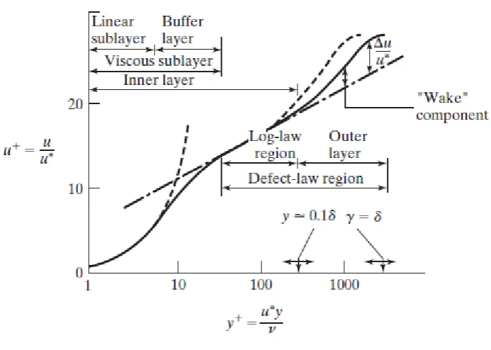
2.6.3 Near-Wall Turbulence
The flow physics of turbulent boundary layers become considerably more complex due to the presence of walls. The mean velocity is affected by the no-slip condition at the wall where the flow is reduced to laminar flow. The near wall zone requires many grid nodes to resolve the variations in flowfield because velocity and other transport properties vary rapidly a short distance from the wall (Pozrikidis, 2017); (Chen, 1997). Turbulent boundary layer along a wall has a substantial region of inertia-dominated flow far away from the wall, but close to the wall flow is influenced by the viscosity of fluid and is independent of freestream parameters (Versteeg & Malalasekera, 2007). At high Reynolds numbers, the viscous part of boundary layer becomes very thin, and as a result it is difficult to use enough grid points to resolve it. This problem can be avoided by using the wall functions that rely on law of the wall of turbulent boundary layer (Ferziger & Peric, 1999).
𝜏 = 𝜇𝜕𝑢
𝜕𝑦− 𝜌𝑢′𝑣′
(2.34)
Numerous experiments have confirmed that near wall region can be divided into outer and inner layers, shown in Figure 2.17. The inner region that accounts for 10-20% of the total thickness of wall layer can be further subdivided into three layers: laminar sublayer, buffer zone and log-law layer (Bertin, 2002). The quantity 𝑢∗that appears in Figure 2.17 is the friction velocity of the fluid that can be described by the following relationship:
𝑢∗= √𝜏𝑤 𝜌
(2.35)
Figure 2.17: Structure of turbulent velocity distribution near a solid wall (Bertin, 2002)
The laminar sublayer is very thin (y+ = 5-10), and it can be assumed that shear stress is approximately equal to wall shear stress 𝜏𝑤 throughout this region (Bertin, 2002).
Therefore, laminar sublayer of the boundary layer can be evaluated as follows:
𝑢+ ≡ 𝑢 𝑢∗ ≈
𝜌𝑢∗𝑦 𝜇 ≡ 𝑦
+ (2.36)
The above equation is called law of the wall, and it contains definitions of two dimensionless parameters used in CFD (Versteeg & Malalasekera, 2007). In the equation,
linear relationship between velocity and distance from the wall in laminar sublayer, the region is known as linear sublayer (Versteeg & Malalasekera, 2007); (Bertin, 2002).
There is an interim region between laminar sublayer and the inner layer, termed as buffer zone in Figure 2.17. This region provides a gradual transition from laminar to fully turbulent regime, therefore effects of viscosity and turbulence are equally important in this region (Versteeg & Malalasekera, 2007). Outside the laminar sublayer turbulent stresses dominate in log-law layer, therefore they must be included to correctly predict the velocity profile of turbulent part of boundary layer (Moran, 2012). By making an assumption regarding the length scale of turbulence, the standard form of log-law layer can be obtained as follows:
𝑢+ ≡ 𝑢 𝑢∗ =
1 𝑘ln 𝑦
++ 𝐶 (2.37)
The number of mesh points required to resolve all the details in a turbulent boundary layer can sometimes be too large. Therefore, wall functions can be used in CFD to bridge the regions between wall and fully turbulent flow when regions affected by fluid viscosity are not resolved by the mesh (Chen, 1997). Wall functions are set of semi-empirical formulas that describe the solution variables at near wall region and the corresponding quantities on the wall. The wall functions constitute law of the wall and near wall turbulent quantities formulas. If the value of 𝑦+is greater than 11.63, the first grid point is considered to be in the log-law region of a turbulent boundary layer. In this region, wall function formula in equation (2.37) that is associated with log-law is used to calculate the shear stress and other
flow variables. However, when 𝑦+ values are lower than 11.63 for grid points adjacent to wall, CFD applies the laminar stress-strain relationship described in equation (2.36)
(Versteeg & Malalasekera, 2007).