Optimal Step Size for the Adaptive Least-Mean Squares Algorithm Applied in the Fractional Fourier Transform Domain for Efficient Signal Estimation in Interference and Noise

(1)

International Journal of Emerging Technology and Advanced Engineering

Website: www.ijetae.com (ISSN 2250-2459,ISO 9001:2008 Certified Journal, Volume 5, Issue 10, October 2015)

29

Optimal Step Size for the Adaptive Least-Mean Squares

Algorithm Applied in the Fractional Fourier Transform Domain

for Efficient Signal Estimation in Interference and Noise

Seema Sud

The Aerospace Corporation, 4851 Stonecroft Blvd. Chantilly, VA 20151

Abstract—The Fractional Fourier Transform (FrFT) has

wide applications in communications and signal processing. It has been shown to provide significant improvement over the conventional Fourier Transform when the signal-of-interest (SOI) or the interference and noise environment is non-stationary, as is often the case. Recently, a Least-Mean Squares (LMS) algorithm was developed for computing the optimum weight vector of the adaptive linear filter applied in the FrFT domain to estimate a SOI from the environment. A computational complexity exists, however, in that typically the FrFT rotational parameter ‘a’ cannot be mathematically computed a priori, and with the LMS algorithm, there is also a step size µ that must be computed. Finding the optimum rotational parameter and optimum step size could require several iterations to achieve the minimum mean-square error (MMSE) for this adaptive filtering method. Since the rotational parameter cannot in general be calculated mathematically, in this paper we develop a method to determine the optimum step size µopt mathematically, thereby improving practical use of the algorithm. We show that the optimum step size produces the MMSE, as desired, and in fact, the step size itself converges to the MMSE as a function of time. We demonstrate the proposed method by simulation of a BPSK signal in non-stationary noise.

Keywords—Adaptive Filtering, Fractional Fourier Transform, Least-Mean Squares, Minimum Mean-Square Error, Step Size.

I. INTRODUCTION

The Fractional Fourier Transform (FrFT) can be applied to a wide range of signal processing problems that occur in quantum mechanics, optics, image processing, data compression, and communications, to name a few applications [11]. For example, it has been applied successfully in place of the FFT in orthogonal frequency division multiplexing to improve performance in channels that are dispersive in both time and frequency [2]. The FrFT allows us to represent signals in a time-frequency plane, rather than just the frequency dimension that the conventional Fourier Transform allows. This enables us to potentially improve our ability to do signal separation or interference mitigation.

Much of the research on FrFT applications has been done in the optics field [3]. Derivation of the optimal linear filter to be used in the FrFT domain was described in [9]. In [10] a least-mean square (LMS) algorithm to implement adaptive filtering in the FrFT domain is introduced. Convergence of the algorithm is discussed, but the choice of optimum step size for the LMS algorithm is obtained by trial and error. Implementation of the LMS algorithm in the FrFT domain is further complicated by the fact that the FrFT rotational parameter „a‟ must usually be computed by trial and error, i.e. by varying „a‟ and choosing the value that gives the minimum mean-square error (MMSE) between a desired signal and its estimate. Since „a‟ cannot be computed mathematically for most problems [9], in this paper we describe a new method for computing the optimal step size, denoted µopt for the FrFT-based LMS algorithm. This allows practical implementation of such an algorithm for better estimation and interference mitigation in the time-frequency space that the FrFT spans.

An outline of the paper is as follows: Section II presents the adaptive filtering problem, in the Fractional Fourier Transform (FrFT) domain. Section III presents the Least Mean-Square (LMS) algorithm for computing the filter solution. Section IV describes the proposed method for computing the optimum step size µopt for this FrFT-based LMS algorithm. We demonstrate that the optimum step size provides the MMSE solution. Section V shows simulation results to study the performance accuracy of the proposed approach. Finally, conclusions and remarks on future work are given in Section VI.

II. ADAPTIVE FILTERING IN FRACTIONAL FOURIER

TRANSFORM (FRFT)DOMAIN

(2)

International Journal of Emerging Technology and Advanced Engineering

30

In general, we seek the M×1 weight vector w(i) that minimizes the error between the estimate of the desired signal and the true desired signal d(i), i.e. we seek to minimize the mean-square error (MSE), defined by [5]

Where we can write the estimate of the desired signal as

The MMSE solution is readily obtained as [7]

Where Rxx(i) = E[xH(i)x(i)] is the well-known covariance matrix of the observed signal and Rxd(i) = E[xH(i)d(i)] is the cross-correlation between the observed and desired signals. The error signal is defined as

As was first proposed in [10], we can perform all of the above operations to improve performance in the presence of non-stationarity by first transforming all of the variables into the Fractional Fourier Transform (FrFT) domain. The FrFT, discussed in numerous papers in the literature, is a transform in the time-frequency plane. It allows signal separation by representing signals in a second dimension, such that even if signals overlap in time or in frequency, there may be a certain rotation factor „a‟ that can be applied in the time-frequency plane such that the signals do not overlap [9]. This enables enhanced signal separation. The FrFT of a function f(x) of order a is defined as [11]

where the kernel Ba(x,x′) is defined as

 = aπ/2, and . This applies to the range 0 < || < π, or 0 < |a| < 2. Denoting the FrFT of order „a‟ of a signal x as Xa, we can write the FrFTs of signals x(i), d(i), and e(i) as Xa(i), Da(i), and Ea(i), respectively [10], where we can explicitly write

The MMSE solution in the FrFT domain is then

Where

and

III. FRFTBASED LMSALGORITHM

The optimum Wiener filter solution cannot be obtained in practice when the statistics of the observed signal are unknown, but we can use a least mean-square (LMS) solution which iteratively updates the weight vector based on an adaptive algorithm [10]. Furthermore, performing the LMS algorithm in the FrFT domain improves the convergence of the weight vector to the optimal solution. We write the update to the weight vector in the FrFT domain, using the LMS algorithm as [10]

Here, µ is a step size that is typically small. However, the optimum step size, µopt, for convergence to the MMSE solution must be obtained by trial and error. The step size range required for convergence, however, is ([6] and [10])

where λmax is defined as the maximum eigenvalue of the matrix RXaXa. In the next section, we propose a method for obtaining µopt.

IV. PROPOSED METHOD FOR COMPUTING OPTIMUM STEP

SIZE OF FRFT-BASED LMSALGORITHM

(3)

International Journal of Emerging Technology and Advanced Engineering

[image:3.612.59.273.145.230.2]

31

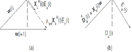
Fig. 1. Vector Representation of Weight Vector Update Equation

Theorem 1: When µ(i) = µopt(i), and as i ⇒ ∞, w(i) ⇒

w

. In other words, when we choose the optimum step size, the weight vector converges to the MMSE solution over time.

Proof: Substitute the value of µopt into Eq. (11) to write

Substituting for Ea(i) from Eq. (7),

As i ⇒ ∞, w(i+1)−w(i) ⇒ 0, as long as the convergence condition in Eq. (12) is followed, so we can write

Solving for w(i) produces the desired result.

Theorem 2: When µ = µopt = E[w H

(i)Xa H

(i)Ea(i)], and as i

⇒ ∞, the MSE approaches the MMSE as defined by Eq. (8) in [10] as

Proof: Again substitute for Ea(i) from Eq. (7) into Eq. (14), rearrange terms (which we can do since Ea(i) is a scalar), and expand

From Theorem 1, as i ⇒ ∞, w ⇒ wMMSE, so substituting using Eqs. (8), (9), and (10),

So,

Now, going back to Eq. (14), write

Rearranging,

Multiplying both sides by E[Xa(i)], we get

Now we rearrange to solve for ||Ea(i)|| 2

, which we recognize as the definition of MMSE.

Substituting for ∂w/∂i from Eq. (21) and cancelling common terms gives the desired result of Eq. (17)

and thus completes the proof.

The following theorem is an interesting result that relates the optimum step size µopt(i) as i ⇒ ∞ to the MMSE.

Theorem 3: µopt(i ⇒∞) = ||Ea,min||2.

Proof: Substituting for Xa(i)w(i) from Eq. (7) into Eq. (13), write

Multiplying both sides by XHa, we get

(4)

International Journal of Emerging Technology and Advanced Engineering

32

Using Eq. (7) again by substituting for Ea(i), we get

Substituting the MMSE solution for w(i), we get

Which from Eq. (17) is the desired result.

V. SIMULATIONS

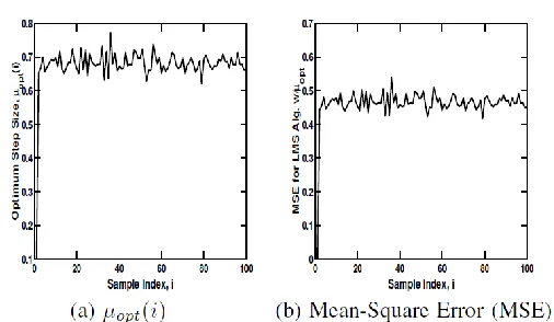
[image:4.612.323.576.130.277.2]

We present simulation examples to demonstrate the validity of Eq. (13) for computing the optimum step size of the LMS algorithm in the FrFT space. The first example is a binary phase shift keying (BPSK) signal in additive white Gaussian noise (AWGN). Since the signal is stationary, we can apply an FrFT with rotational parameter a = 0, which simplifies to the time-domain signal itself [11]. We choose the noise variance such that the signal-to-noise ratio (SNR) is 10 dB. This is set by setting the signal amplitude equal to one, and setting the noise variance to σN2_{= 10}−SNR/10_. Figure 2a shows µopt(i) vs. the time sample, i, for i = 1,2,3,...,1000. Because of the simple scenario, µopt(i) converges quickly, after just a few samples. If we average over T = 100 samples to satisfy the expectation criteria of computing actual µopt values from Eq. (13) and in all the other equations, we see that it converges to an average value of µopt,100 = 0.66. The corresponding MSE, i.e. ||Ea(i)||2, is plotted in Figure 2b. The averaged MSE over the last 100 samples, similarly, is MSEave,100 = 0.52, which agrees closely with µopt,100, thereby validating Theorem 3. Furthermore, the MSE closely agrees with the MMSE, computed from Eq. (17) as MMSEave,100 = 0.47 (note that the values all agree to within about 1 dB, differences being due to noise, estimation errors, lack of statistical observations, etc.). Since our choice of step size results in an MSE that equals the MMSE, this shows that we have found the optimum step size (refer back to Theorem 2).

Fig. 2. Performance of LMS Algorithm with Optimal Step Size; BPSK Signal in AWGN; SNR = 10 dB

We note that the algorithm is not sensitive to the initial choice of w(i = 1) or µ(i = 1); we let the initial weight vector be all zeros and took µ(i = 1) = 0.001 in this example, much smaller than the actual value turns out to be. Choosing the initial weight vector to be the unit vector, or choosing µ(i = 1) = 0.01 or 0.1 did not make much difference in the final value of µopt(i ⇒ ∞) or the corresponding MSE. Note also that as another check on µopt(i), we can compute the maximum value of µ required for convergence. In this case it is λ/2 = 4.84, so the value of µopt clearly falls in the range required for convergence.

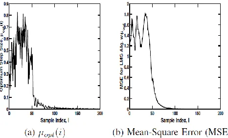
In the second example, we again consider a BPSK signal as defined above, but this time we let the noise be a nonstationary process defined by the chirp signal

Where fs is the sampling rate, which we set to 10, and i/fs is time. This is the same noise process applied in the example in [9], Eq. (3). We further set a = 0.5, as is shown in the example to provide the best performance. Again, µopt(i) and the MSE converge quickly, after just a few samples, so we plot only 200 samples in Figure 3. We again average over the last T = 100 samples to obtain an average value of µopt,100 = 4.7 × 10−3. The corresponding average MSE, i.e. ||Ea(i)||

2

, is MSEave,100 = 2.7 × 10 −3

(5)

International Journal of Emerging Technology and Advanced Engineering

[image:5.612.327.576.130.277.2]

33

Furthermore, the MSE again closely agrees with MMSEave,100 = 1.8×10−3. Note that the MSE and MMSE is better than in the previous example. This is because we can apply the FrFT to separate the noise and interference, which do not overlap as much in the a = 0.5 domain as they do in the time domain (a = 0). If we apply a = 0 here as in the previous example, the MSE is worse than in the previous example.

Fig. 3. Performance of LMS Algorithm with Optimal Step Size; BPSK Signal in Non-Stationary Noise; SNR = 10 dB

[image:5.612.56.289.236.377.2]

The third example uses the same signal and noise process as in the last example. But, now we also have a second interfering BPSK signal. The amplitude of the first signal is set to one as before, and the amplitude of the second signal is set to A2 = 10−CIR/10, where CIR is the carrier-to-interference ratio between the first signal and the interfering one. In this example, we let CIR = 5 dB, so that A2 = 0.316. Figure 4a shows 200 samples of µopt(i), and the value converges to µopt,100 = 5.0 × 10−3. The corresponding MSE, i.e. ||Ea(i)||

2

, is plotted in Figure 4b, and MSEave,100 = 3.1×10−3, and MMSEave,100 = 2.0×10−3. Performance in this example is worse than in the previous example because of the stationary interferer but it still performs well due to the reasonably high CIR and the use of a training signal d(i).

Fig. 4. Performance of LMS Algorithm with Optimal Step Size; BPSK Signal in Interference and Non-Stationary Noise; SNR = CIR = 10 dB

Note that in the above examples, we need the best value of „a‟, which is usually found by minimizing the MSE between a training signal and its estimate. Finding other methods to determine the best „a‟ is the subject of ongoing research.

VI. CONCLUSION

In this paper we propose a method for computing the optimum step size µopt for the LMS algorithm applied in the Fractional Fourier Transform (FrFT) domain. We show that the choice of optimum step size results in the LMS algorithm weight vector converging to the MMSE solution, and that the optimum step size itself approaches the MMSE. We demonstrate the validity of these results by simulation using BPSK signals in AWGN, non-stationary chirp noise, and a co-channel BPSK signal. Future work includes developing methods to estimate the optimum rotational parameter „a‟.

Acknowledgments

(6)

International Journal of Emerging Technology and Advanced Engineering

34

References

[1] Almeida, L.B., “The Fractional Fourier Transform and

Time-Frequency Representation”, IEEE Trans. on Sig. Proc., Vol. 42, No. 11, Nov. 1994.

[2] Azmy, M.H., Elgamel, S., Mamdouh, A., and El-Barbary, K.,

“Performance Improvement of the OFDM System Based on Fractional Fourier Transform over Doubly Dispersive Channels”, Proc. IEEE Int. Conf. on Engineering and Technology, Cairo, Egypt, Oct. 10-11, 2012.

[3] Bultheel, A., and Sulbaran, H.E.M., “Computation of the Fractional

Fourier Transform”, Int. Journal of Applied and Computational Harmonic Analysis 16 (2006), pp. 182-202.

[4] Gardner, W.A., Napolitano, A., and Paura, L., “Cyclostationarity:

Half a Century of Research”, EURASIP Int. Journal of Advances in Sig. Proc. 86 (2006), pp. 639-697.

[5] Goldstein, J.S., and Reed, I.S., “A New Method of Wiener Filtering

and its Application to Interference Mitigation for Communications”, Proc. of IEEE MILCOM, Vol. 3, pp. 1087-1091, Monterey, CA, Nov. 1997.

[6] Haykin, S., “Adaptive Filter Theory”, Prentice Hall: Upper Saddle River, New Jersey, 1994.

[7] Honig, M.L., and Poor, H.V., Adaptive Interference Suppression. In

Poor, H.V., and Wornell, G.W., editors, “Wireless Communications: Signal Processing Perspectives”, Prentice Hall: Englewood Cliffs, New Jersey, pp. 64-102, 1998.

[8] Huang, Y., Benesty, J., and Chen, J., “Optimal Step Size of the Adaptive Multichannel LMS Algorithm for Blind SIMO Identification”, IEEE Sig. Proc. Letters, Vol. 12, No. 3, Mar. 2005.

[9] Kutay, M.A., Ozaktas, H.M., Arikan, O., and Onural, L., “Optimal

Filtering in Fractional Fourier Domains”, IEEE Trans. on Signal Processing, Vol. 45, No. 5, May 1997.

[10] Lin, Q., Yanhong, Z., Ran, T., and Yue, W., “Adaptive Filtering in

Fractional Fourier Domain”, International Symposium on

Microwave, Antenna, Propagation, and EMC Technologies for Wireless Communications Proc., pp. 1033-1036, 2005.

[11] Ozaktas, H.M., Zalevsky, Z., and Kutay, M.A., “The Fractional