Cooperative Control of Multiple Quadrotors for Transporting a Common Payload

AUT J. Model. Simul., 50(2) (2018) 147-156 DOI: 10.22060/miscj.2018.14252.5100

Cooperative Control of Multiple quadrotors for Transporting a Common Payload

R. Babaie, A. F. Ehyaei*

Department of Electrical Engineering, Imam Khomeini International University, Qazvin, Iran

ABSTRACT: This paper investigates the problem of controlling a team of quadrotors that cooperatively transport a common payload. The main contribution of this study is to propose a cooperative control algorithm based on a decentralized algorithm. This strategy is comprised of two main steps: the first one is calculating the basic control vectors for each quadrotor using Moore–Penrose theory aiming at cooperative transport of an object and the second one is combining these vectors with individual control vectors, which are obtained from a closed-loop non-linear robust controller. In this regard, a nonlinear robust controller is designed based on Second Order Sliding Mode (SOSMC) approach using Extended Kalman-Bucy Filter (EKBF) to estimate the unmeasured states which is capable of facing external disturbances. The distinctive features of this approach include robustness against model uncertainties along with high flexibility in designing the control parameters to have an optimal solution for the nonlinear dynamics of the system. Design of the controller is based on Lyapunov method which can provide the stability of the end-effecter during the tracking of the desired trajectory. Finally, simulation results are given to illustrate the effectiveness of the proposed method for the cooperative quadrotors to transport a common payload in various maneuvers.

Review History:

Received: 28 March 2018 Revised: 19 October 2018 Accepted: 22 October 2018 Available Online: 25 October 2018

Keywords:

quadrotor

Second Order Sliding Mode Control Extended Kalman-Bucy Filter Cooperative Decentralized Control External Disturbances

1- Introduction

The cooperative control of multiple vehicle systems despite its wide range of practical applications requires tackling important theoretical and practical challenges which have attracted many researchers in recent years. Formation control problems for multiple vehicle systems can be categorized with applications to unmanned aerial vehicles (UAVs), autonomous underwater vehicles, cooperative transport, mobile robots, cooperative role assignment and cooperative search. In this paper, we seek to drive a control algorithm for cooperation between quadrotors that allow the robots to control their position and angles to grasp and transport a common payload in various maneuvers. The controller is designed to move the object by two or more quadrotors. To make a framework for interplay between a group of quadrotors and payload, many control schemes have been extensively used to solve the problems of creating formation control for UAVs. Some of them have focused on centralized and leader-follower approach to access interaction between cooperative quadrotors and payload [1-7]. Although these methods have acceptable results on small robotic systems but suffer from several disadvantages including high computational complexity of centralized methods in large-scale systems and possibility of disappearing the group formation in leader-follower strategy due to not receiving the position of leader by the followers.

In this regard, there is a plethora of research in cooperative multi-robot controller design based on decentralized control methods which can solve a significant number of problems in cooperative control strategies and benefit also from the

advantages such as decreased number of sensors and fast performance. In [8], the problem of cooperation by a team of ground robots is addressed under quasi-static assumptions based on decentralize controllers considering a unique solution to robot and object motion. Also, transporting a payload by aerial manipulation using cables based on decentralized control is studied in [9,10]. In other research, cooperative aerial towing-based decentralized mechanism is studied [11]. The authors of [12] employ bilinear matrix inequalities to present optimal solutions for decentralized nonlinear multi-agent systems. Despite the numerous advantages of decentralized methods, there are still some critical issues related to the performance of the control system in presence of disturbances and uncertainties.

approach, the performance of control system was improved by using a second-order sliding mode control (SOSMC) for second-order uncertain plants. An adaptive SOSMC with a nonlinear sliding surface was introduced in [23] and a linear switching surface was proposed for similar underactuated systems in [24]. Wind as a disturbance source has also been considered in the flight process of the quadrotor to demonstrate the robustness of the control algorithm [25,26]. So, SOSMC is a suitable method for controlling uncertain (and possibly disturbed) nonlinear systems, specially UAVs, where the necessity of robust tracking schemes, as well as fast convergent algorithms is crucial.

Hence, in this paper, a decentralized robust optimal controller is designed for a group of UAVs in a formation which enables manipulation of a common payload in three dimensions. Our cooperative control algorithm is comprised of two parts. In the first part, basic control vectors, which guarantee the optimal performance of the coupled system, are determined using Moore-Penrose theory. In the second part, individual control vectors are designed for each quadrotor which can guarantee robustness of the coupled system against uncertainties and disturbances. Moreover, a combination of second order sliding mode controller with an optimal cooperative algorithm is employed to control all the quadrotors such that a soft touching occurs between the object being carried and the cooperative quadrotors. A nonlinear filter equivalent to well-known Extended Kalman-Bucy filter (EKBF) in a continuous-time stochastic system has also been developed in our work to improve the estimation accuracy and robustness of the system. The simple design and implementation and accurate estimation of state variables under noisy condition make EKBF suitable for robotic manipulators and other industrial applications.

Finally, the proposed controller successfully rejects the external disturbances (e.g. wind effect) for cooperative quadrotors. The other advantages of using this approach are from simple implementation and flexible parameter learning to design criteria customization. The simulation results show the effectiveness and superior performance of the proposed control strategy for transporting a common payload in various maneuvers by cooperative quadrotors.

The subsequent parts of this paper are as it follows. First of all, developing a model for a single quadrotor and modeling of a team of UAV’s rigidly attached to a payload is discussed in Section 2. In Section 3, the Extended Kalman Bucy Filter is described briefly. Section 4 proposes cooperative control algorithms defined with respect to the payload that

stabilizes the object along three dimensional trajectories based on a SOSMC incorporated with optimal Moore-Penrose theory. We review and analyze experimental study with teams of quadrotors cooperatively grasping, stabilizing, and transporting payloads in Section 5. It includes point-to-point path planning and trajectory tracking. Finally, Section 6 concludes the paper with some future improvement suggestions.

2- Mathematical Modeling and Coordinate Reference Frame

2- 1- Dynamic Model of single quadrotor

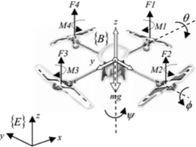
Fig.1 shows the configuration of our quadrotor system that can fly in all directions and has no limit on maneuver. Two main reference frames are considered: model frame, E=

{

E E Ex, ,y z

}

, and the body-fixed reference frame, B=

{

B B Bx, ,y z

}

. In this nomenclature, ξ

[

, ,

]

T

x y z

= and _η=

[

_{ϕ θ}, ,_Ψ

]

T _{are the position} and orientation vectors in reference E. F ii

(

=1,2,3,4

)

is

the thrust force produced by four rotors. The full quadrotor dynamical model with the , ,x y z motions as outcome of a pitch, roll and yaw rotation is [27]:

(

)

(

)

¨ ¨

2 ₁

¨ ¨

3 1

¨ ¨

4

x

x _i

y i

Iy Iz jr l _{U x cos sin cos sin sin} l _U

Ix Ix I m

Iz Ix jr l_{U y cos sin sin sin sin} l _U

Iy Ix y m

Ix Iy l_{U z g cos c}

Iz Iz

ϕ

θ

ψ

ϕ θψ θ ω ϕ θ ψ ϕ ψ ω

θ ϕψ ϕ ω ϕ θ ψ ϕ ψ ω

ϕ

ψ ϕθ ω

 ₌  − _{− Ω + +}

= + +

 

 _{ }



 _{ − }

 = − Ω + + = − +

  

 



 _{ − }

= − +

 = _{ }+ +

 



_ 

  





(

)

1 z

i

l os U

m

θ ω

      

+ 



(

)

(

)

¨ _¨

2 1

¨ ¨

3 1

¨ ¨

4

x

x _i

y i

Iy Iz jr l_{U l}

x cos sin cos sin sin U

Ix Ix I _m

Iz Ix jr l_{U y cos sin sin sin sin} l _U

Iy Ix y m

Ix Iy l _{U z g cos c}

Iz Iz

ϕ

θ

ψ

ϕ θψ θ ω _{ϕ θ ψ ϕ ψ ω}

θ ϕψ ϕ ω ϕ θ ψ ϕ ψ ω

ϕ

ψ ϕθ ω

 ₌  − _{− Ω + +}

= + +

 

 _{ }



 _{ − }

 = − Ω + + = − +

  

 



 _{ − }

= − +

 = _{ }+ +

 



_ 

  





(

)

1 z

i

l

os U

m

θ ω

      

+ 



(1)

where

2

1 1

2

2 2

2

3 3

2

4 4

0 0

0 0

b b b b

U

lb lb

U

lb lb

U

k k k k

U

 

 

   

  _Ω

   

  ₋

   

  = Ω

 −  

 

Ω

   

  _{− −}

 _{  }

  _Ω

   _,

(2)

in whichm_i is considered as mass of one quadrotor; also k

and b represent the thrust and drag coefficient, respectively. The input U₁ is related to the total thrust; while the inputs

2, ,3 4

U U U are related to the rotations of the quadrotor and

, , , , , x y z ϕ θ

ω ω ω ω ω ωΨ are external disturbances,

jr

denotes

the inertia of the z-axis and Ω = −Ω + Ω − Ω + Ω_{1 2 3 4} is the overall residual propeller angular speed. The model in Eq. (1) can be rewritten in a state-space form, X = f

(

X,U

)

, where

[

1, .., 12

]

, , , , , , , , , , , ÿ

T

x x y y z z

ϕ ϕ θ θ ψ ψ

 

= …… _{=  }

     

X x x T

is the state vector of the system.

Assumption 1 .It is assumed that the roll ,pitch and yaw angle satisfy the conditions ϕ

( )

t / 2 <π ,θ

( )

t / 2<π

,

and ψ π< for t ≥ 0

2- 2- Dynamic Model of Coupled System

According to Fig.2 , we consider a group of 4 quadrotors jointed through a fixed interaction to the cross object coordinate frame B. The axes of the coupled system are described as body frame axes and each UAV has an individual body frame Qi where i=

{

1,2, ,…n

}

and nis the number of

UAVs in the group. For extracting the dynamic model of the coupled system we assumed the quadrotors are rigidly connected to the object and also, the center of mass of the system is intended as the origin of the rigid-body coordinate system. Therefore, the motion formulation for each quadrotor can be written as:

¨ Qi

i i B

m z = −m g+F_i , (3) where FBi is lift force generated by each quadrotor. By

applying Newton’s second law to the payload, we have: ¨

QB

i L

m Z = −m g , (4) where mL is the mass of the object. Since, all the forces are

used for lifting and moving toward the positive Z direction, the equation of motion for the coupled system can be easily written as:

B, 1 2 3 4 L

mz= −mg+F m m m m m m= + + + +

1 2 3 4

m m m m m= + + + + (5) which

F

_B is the total lift force imposed by all quadrotors and

m

is sum of the quadrotors and object’s mass. Hence, the rotor forces can be rewritten as a total force from each quadrotor

F

_{q i,} . By considering each UAV’s generated forces and moments in its own frame, we need to develop a relationship between the behavior of the system and the agents. Finally, the equation of motion for the coupled system is obtained as it follows [28]:

,

,

,

,

1 0 0 0

sin 0

sin 0

0 0 0 1

B

B

B

q i

xq i

i i i

i

yq i

i i i

i B

zq

x y cos

x cos

y z

ψ ψ

ψ ψ

  _{ }

 

  _{ }

 

  _{−  }

 

=

  _{ }

− 

  _{ }

 

  _{   }

 

 

∑

F

M _M

M M M

F

M (6)

where MxB, My B, Mz B are the body moments in the ZQi direction as shown in Fig. 2. Also, F_{q i,} is the total force from each quadrotor and M_{xq i,}, M_{yq i,}, M_{zq i,} are moments around each quadrotor’s body frame axis.

3- Nonlinear Observer Based on EKBF

The Extended Kalman Bucy Filter is considered as an optimal recursive estimation algorithm for calculating the states of a nonlinear stochastic system with uncorrelated Gaussian process and measurement noise. EKBF is designed by determining the filtering and prediction equations. Consider a nonlinear stochastic system with uncorrelated Gaussian process and measurement noise as it follows [29-31]:

( )

(

( )

)

( ) ( )

d tx =f x t , t dt G t d t , t+ w ∀ ∈

(

)

k= k, tk + k

Z h x v (7)

where x

( )

t is the state vector and Zk is the measurement vector. w

( )

t and v_k denote the state and measurement noise, a noise that apply to the system state variables in kalman filter process. In filtering step, the estimation of error covariance matrix is determined by:

(

) (

) (

)

´ ´ T ´ ´ ´ ´

k = k− k ˆk, tk ˆk, tk ˆk, tk k

P P P H x K x H x P (8)

The estimated parameters by kalman filter have indicated by notation prime. and Kalman filter gain is computed as:

(

_´

)

(

_´

)

_{´ T}

(

_´

)

1

k k k k k k k k

ˆ , t ₌ ˆ , t ˆ , t ₊ −

 

K x H x P H x R (9)

where Rk represents the covariance matrix of the sensor noise. In prediction step, we have:

( )

₍

_{( )}

₎

´

´ d t

t , t

dt ˆ

ˆ

=

x _{f x (10)}

( )

₍

´

_{( )}

₎

_{( )}

_{( )}

T

₍

´

_{( )}

₎

_{( )}

d t

t , t t t t , t t

dt = ˆ + ′ ˆ +

′

′

P _{F x P P F x Q (11)}

where _{F x}

(

_ˆ´

( )

_{t , t}

)

_and

(

´

)

k k

ˆ , t

H x are the Jacobean matrixes of f x

(

( )

t , t

)

and h x

(

_k, t_k

)

evaluated at _xˆ´

( )

_{t respectively.} Moreover, Q

( )

t represents the power of measurement noise. After applying EKBF on system, the estimated is shown as

[

1 12

]

ˆ ˆ

ˆ _{ˆ ˆ ˆ ˆ ˆ ˆ ˆ ˆ ˆ ˆ ˆ ˆ}

,= …….., _{= }ϕ ϕ θ θ ψ ψ, , , , , , , , , , , x x y y z z_T

      

x x T

X ,

where _Xˆ_∈4 4n× _{is a constant vector containing the states of} translational and rotational subsystems.

Remark 1. Usually, in a real application, the “true” states are not available and the states are estimated from the measurement system. To design the controller based on the “estimated” states using a Kalman filter, although the choice of the assumed covariance matrices Q and R can have a significant effect on the estimation performance, it is also necessary to decrease the sampling time sufficiently. In this regard, one can observe that both parameters Q and R have a direct relation with sampling time which means that lowering the sampling time leads to a decrease in the estimation error and directs the estimated values toward the “true” states. Therefore, in this paper, in order to ensure that the “true” states converge to the desired values using the estimated states, the following conditions will be considered based on simulations:

( )

1 00000; ≥ , 0.0001; ≤

N number of time steps, dt Sampling time s

( )

1 00000; ≥ , 0.0001; ≤

N number of time steps dt Sampling time s ,

(

)

( )

* 1:= ;

t dt N timevector s

upper limit of input frequency of the desired value (i.e. 0.5Hz in this paper). This computational method is based on trial and error strategy to minimize an ITAE cost function of estimation error.

4- Cooperative Control Strategy

In this section, the perfect state cooperative guidance controller of UAV presented in [28] will be developed to achieve a decentralized control strategy with superior results regarding state estimation. Therefore, the problem considered in this part is separated in two steps: the first step focuses on designing the basic control vectors for n quadrotors using the Moore-Penrose theory based on estimated state variables which are generated by EKBF, and the second step describes how to determine individual control vectors by SOSMC. Finally, the cooperative control algorithm can be extracted by combining the individual control vectors and the basic control vectors.

4- 1- Deriving Basic Control Vectors of Cooperative Control Law

By using all force vectors of the coupled system in linear system (6), four equations for 4 quadrotors can be established as follows:

, , , T ˆ

B xB yB zB u

  =

F M M M  X (12)

where _u∈4n _{includes 4 control input vectors for each n} quadrotor:

,1 ,1 ,1 , , ,

,1, ,Bq Bq , Bq .., , , ,Bq n q n, q n T

Bq x y z Bq n x yB zB

u=_F M M M … F M M M _ (13) Now, consider the following cost function to minimize the control inputs [28]:

(

, , ,

)

2 2 2 2

, q i q i q i

Fi q i Mxi x Myi y Mzi z i

J =

∑

Λ F + Λ M + Λ M + Λ M ₍₁₄₎

in which Λ ΛFi, Mxi,ΛMyi,ΛMzi are the weight of each of the control inputs. By considering the features of mathematical theory of Moore-Penrose inverse, point-wise minimization of the function J will be accrued and an optimal control vector can be written as [28 ]:

* 2 ˆT₍ ˆ 2 ˆT₎1 des_, des_, des_, des T

B xB yB zB

u _{= Γ}− X X_Γ− X − _F M M M _

  (15)

where: 2 2

u

Γ = Γ ,

1, 1, 1, 1,..., , , ,

F Mx My Mz Fn Mxn Myn Mzn

dig 

Γ = _ Λ Λ Λ Λ Λ Λ Λ Λ _,

by assuming the weight of basic control vectors

,

Fi F Mxi Myi Mzi

Λ = Λ Λ = Λ = Λ , we have,

(

)

1

2ˆ ˆ 2ˆ _{, , ,}

qn qn qn qn

T T

F Mz Mx My

X X X − U U U U

− − _{ }

Γ Γ _{=  .}

Also, according to this fact that all quadrotors have a common role in lifting the object off the ground and equal partnership, the body force F and yaw torque produced by each of them is almost equal. Therefore, the basic control vectors which include total force, yaw, pitch and roll moment generated for the coupled system structure are obtained as follows:

[ ]

[ ]

1 1 1

2

1 1 1

2

1 1,0,0,0, ..,1,0,0,0 1 0,0,0,1, ,0,0,0,1

1 _{, , ,0, , , , ,0}

1 _{, , ,0, , ,}

qn qn qn qn

z Mxy Mxy

q q q qn qn qn

Mxy F F

i F y

Mxy Mxy

q q qn

Mxy F F

i F

n

U _n

U _{y C S y C S}

U _{y n}

U

x S q C x x n ψ ψ ψ ψ ψ ψ … ……     Λ Λ     _… =     _{Λ Λ Λ}     ∑ + Λ       _{Λ Λ} − − … − Λ _{∑ +} Λ Λ Λ F M Mx M , ,0 qn qn

Sψ Cψ

                     _{ }   −   _{ }     (16)

Therefore, four basic control vectors for n cooperative quadrotors obtained according (16) and in the in the next section the individual control vectors, des_qn, des_qn, des_qn, des_qn T,

B xB yB zB

 

F M M M 

will be established. Finally, by combination of two set of mentioned vectors, the cooperative control vectors will be defined as it follows:

, , , , , ,

qn qn qn qn qn qn qn qn

n

T

des des des des

z y B xB yB zB

coop Q

U _{= }U U U U   

  

F M Mx M F M M M (17)

4- 2- Deriving Individual Control Vectors of Cooperative Control Low

In this section, determining individual control vectors of cooperative control strategy based on second order sliding mode technique is supposed to asymptotically perform position and attitude tracking of the quadrotors in order to generate a robust solution. Now, to complete the cooperative algorithm, using tracking errors of state variable(s), a switching sliding surface is considered for the whole subsystem (rotational or transitional). The sliding manifolds based on SOSMC are chosen as it follows [32, 33]:

(

)

(

)

ˆ 1ˆ d ˆ 2ˆ d ˆ

Sϕ=α ϕϕ −ϕ α+ ϕ ϕ −ϕ

(

)

( )

ˆ 1ˆ d ˆ 2ˆ d ˆ

S_θ=α θ_θ −θ +α θ_θ  −θ

(

)

ˆ 1ˆ d ˆ 2ˆ( d ˆ)

Sψ =α ψψ −ψ +α ψψ  −ψ

(

)

(

)

ˆ 1ˆ ˆ 2 ˆ

x x d x d

S =α x −x +α x −x

(

)

(

)

ˆ 1ˆ ˆ 2ˆ ˆ

y y d y d

S =α y −y +α y −y

(

)

(

)

ˆ 1ˆ ˆ 2ˆ ˆ

z z zd z z zd z

S =α − +α  −

(18)

in which, α α1ϕˆ, , ,2ϕˆ…α α1ˆz, 2zˆ>0. The time derivatives of the

sliding manifolds of rotational subsystem are obtained as it follows;

(

)

(

)

ˆ 2

ˆ 1 d ˆ ˆ d ˆ

Sϕ=αϕ ϕ −ϕ α + ϕ ϕ −ϕ

( ) ( )

2

ˆ 1ˆ d ˆ ˆ d ˆ

S_θ=α θ θ_θ  −  +α θ θ_θ  −

(

)

2

(

)

ˆ 1ˆ d ˆ ˆ d ˆ

Sψ =α ψψ  −ψ +α ψψ  −ψ

(19)

By generating Sxˆ= −κsgn

( )

Sxˆ − ΥxˆSˆx , with withxˆ=ϕ θ ψˆ, , ,and 1,2,3 , ˆ ˆ ∈

[

]

( )

ˆ

[

]

xˆ = −κsgn ˆ − Υxˆ , with ˆ=ϕ θ ψˆ, , ,and 1,2,3 , ˆ ˆ ∈

 _{x x }

S S S x  the associated control inputs are

defined as:

(

)

( ) 1 2 1 2 ˆ ˆ ˆ ˆ 2 ˆ ˆ 1 ˆ ˆ

ˆ ˆ sgn

x

d d

I Iy Iz jr

U S S

l Ix Ix

ϕ ϕ ϕ ϕ ϕ ϕ ϕ α ϕ ϕ ϕ θψ θ κ ω α α  −     _{ }  = _ − + − _ _+ Ω +  + Υ − _      _  

( )

( ) ˆ 1 ˆ ˆ ˆ 3 2 ˆ ˆ 2 2 1

ˆ ˆ ˆ ˆ sgn

y

d d

I Iz Ix jr

U S S

l θ Iy Ix θ θ θ θ

θ θ α θ θ θ ϕψ ϕ κ ω α α   −    _{ }  = _ − + − _ _+ Ω +  + Υ − _        

(

)

( )

ˆ 1 4 3 2 2 ˆ ˆ ˆ ˆ ˆ 1 ˆ

ˆ ˆ [ sgn ]

z

d d

I Ix Iy

U _l ψ _Iz S S

ψ ψ ψ ψ ψ ψ α ψ ψ ψ ϕθ κ ω α α  −      =  − + − _ _+ + Υ −           (20)

where κ κ κ₁, , ,_{2 3} Υ Υ Υ >ϕ_ˆ, ,θ_ˆ ψ_ˆ 0 . Now for transitional subsystem, the objective is to guarantee the state variables

respectively. The time derivatives of the sliding manifolds of rotational subsystem are obtained,

ÿ ¨ ¨

1 2

ˆ ˆ ˆ ˆ d ˆ x=αx_ d − _+α x_ − _

 _

S x x x x

ÿ ¨ ¨

1 2

ˆ ˆ ˆ ˆ ˆ ,

y=αy_ d − _+α y_ d− _

 _

S y y y y

ÿ ¨ ¨

1 2

ˆ ˆ ˆ ˆ d ˆ . z =αz_ d− _+α z_ − _

 _

S z z z z

(21)

By generating Sxˆ = −κsgn

( )

Sxˆ − ΥxˆSxˆ ,

(

xˆ ˆ ˆ ˆ=x y z, ,

)

and by considering 4,5,6 , ∈

[

]

the associated control inputs are defined as:

(

)

( )

2 ˆ ˆ ˆ ˆ ˆ ˆ ¨ 1 4 1 2 1 ˆ sgn x _d

x d x x x x

x x

m

U α x x x κ S S ω

µ α α  _{ }  =  − + +  + Υ −      ,

(

)

( )

ˆ ˆ ˆ ˆ ¨ 1

2 2ˆ 5

ˆ

2

1

ˆ sgn

y

y d d y y y y

y y

m

U α y y y κ S S ω

µ α α    _{ }  =  − + + _ + Υ _−        ,

(

)

( )

ˆ ¨ 1 1 6

3 2 2

ˆ

ˆ ˆ ˆ ˆ

1

ˆ [ sgn ]

z _d

d z z z z

z z

m

U α z z z g κ S S ω

µ α α

 

=  − + + + + Υ − 

   _,

(22)

where κ κ κ4, , , ,5 6 Υ Υ Υ >xˆ yˆ, zˆ 0. In addition, the terms µ µ µ1, ,2 3

are:

(

)

(

)

2 cos sin sinˆ ˆ ˆ sin sin , 1 cos sin cosˆ ˆ ˆ sin sinˆ ˆ , 3 cos cosˆ ˆ

µ = ϕ θ ψ− ϕ ψ µ = ϕ θ ψ+ ϕ ψ µ = ϕ θ

(

)

(

)

2 cos sin sinˆ ˆ ˆ sin sin , 1 cos sin cosˆ ˆ ˆ sin sinˆ ˆ , 3 cos cosˆ ˆ

µ = ϕ θ ψ− ϕ ψ µ = ϕ θ ψ+ ϕ ψ µ = ϕ θ (23)

To synthesize a stabilizing control law by second order sliding mode, the sufficient condition for stability of the system, i.e. V

( )

Sxˆ =Sxˆ. .Sxˆ< − Sxˆ, where ℒ is the positive

value (>0), must be verified. The time derivative of V

( )

Sˆx

satisfies Sxˆ. 0Sxˆ< . Thus, a Lyapunov function can be written

as V = ∑1₂S SxˆT ˆx, that one can describe as :

( )

ˆ 1

(

ˆ ˆ ˆ ˆ ˆ ˆ ˆ ˆ ˆ ˆ ˆ ˆ

)

V

2 xT x yT y Tz z ϕT ϕ θT θ ψ ψT

= + + + + +

x

S S S S S S S S S S S S S

. (24) The chosen law for the attractive surface is the time derivative of

( )

ˆ ˆ xˆ ˆ xˆ 2ˆ

V S_x =S_x. S = −κ_S_x − Υ Sx 0≤ (25)

Therefore, according to (25) the time derivative of final Lyapunov function V

( )

Sˆx is as:

( )

(

)

2 2 2

ˆ ˆ ˆ ˆ ˆ ˆ ˆ ˆ ˆ

4 5 6

ˆ _{2 2 2}

ˆ ˆ ˆ ˆ ˆ ˆ ˆ ˆ ˆ

1 2 3

2

ÿ ¨

ˆ ˆ ˆ ˆ

4 1 2 1

ˆ ˆ ˆ

5 1

ˆ

ˆ ˆ ˆ ˆ

ˆ cos sin cos sin sin

x x x y y y z z z

x

d

x x x d x x

y y

S S S S S S

V S

S S S S S S

l

S x x x _mU

S ϕ ϕ ϕ θ θ θ ψ ψ ψ κ κ κ κ κ κ κ α α ϕ θ ψ ϕ ψ ω κ α − − Υ − − Υ − − Υ    = = − − Υ − − Υ − − Υ          − − Υ  _ − _+  −_ + + _     − − Υ   ( )

(

)

(

)

2 ¨ ˆ 2 1 2 ÿ ¨ ˆ ˆ ˆ ˆ

6 1 2 1

ÿ

ÿ ¨ ÿ

ˆ ˆ ˆ ˆ

1 1 2

ˆ

ˆ ˆ ˆ ˆ

ˆ cos sin sin sin sin

ˆ ˆ

ˆ cos cos

ˆ

ˆ ˆ

y d y d y

d

z z z d z z

d d

l

y y y _mU

l

S z z z g U

m

Iy Iz jr

S Ix ϕ ϕ ϕ ϕ α ϕ θ ψ ϕ ψ ω κ α α ϕ θ ω κ α ϕ ϕ α ϕ θψ  _{− +}  ₋ _{− +}    _ _           − − Υ  _ − _+  − − + +        −     − − Υ _ − _+ − _{ }−       2 ÿ 2 2 ÿ ¨ÿ ÿ ÿ ˆ ˆ ˆ ˆ

2 1 2 3

ÿ ¨ ÿ

ˆ ˆ ˆ ˆ

3 1 2 4

ˆ ˆ ˆ ˆ ˆ ˆ ˆ ˆ x d d d d l U Ix I

Iz Ix jr l

S U

Iy Ix y

Ix Iy l

S U Iz Iz ϕ θ θ θ θ θ ψ ψ ψ ψ ψ θ ω κ α θ θ α θ ϕψ ϕ ω κ α ψ ψ α ψ ϕθ ω     Ω + +  _  _  _{  }         −   − − Υ  _ − _+ _ −_{ } _− Ω + + __     −     − − Υ _ − _+ −  + +      2        _{ }   (27)

Thus, under the control laws extracted from SOSMC approach

(

U1, ., , ,… U U U4 x y

)

, all the system state trajectories can reach

at and stay on the associated sliding surfaces, respectively, and guarantees asymptotic stability of closed loop system.

Remark 2. Note that signum function which appears in second order sliding mode controllers and filters can cause chattering phenomena, or high-frequency oscillations of control variables. This problem can be avoided by replacing discontinuous signum function with an appropriate continuous approximation such as sign s

( )

i ≈tanh s

(

i/εi

)

.

Finally, individual control vectors in (20) and (22) that are generated using SOSMC method, represented by parameters which are equivalent of ( des_, , des_{q n,}, des_{q n,} , des_{q n,} )

q n x y z

F M M M . Thus the

individual control vectors for cooperative strategy are defined as follows:

( )

11 11 11

ÿ

ˆ

6 ˆ ˆ ˆ

ˆ ¨ 1 ₁₂ , 3 2 tan ˆ _h

qn qn qn

des z _{qn d}

q n d X X X z

z

m

F α z X z g κ S S ω

µ α       =   − + + + + Υ −        

( )

,

1 1 1

ÿ ¨ ÿ ÿ

ˆ 1

2 3 5

ˆ 2

ÿ

3 1 ˆ ˆ ˆ

ˆ 2 ˆ ˆ ˆ 1 ˆ _tanh q n

qn qn qn

qn _d qn qn

d

des x

x

qn _{X X X}

Iy Iz

X X X

I Ix

M _jr

l _{X S S}

Ix ϕ ϕ ϕ ϕ α _{ϕ ϕ} α κ ω α   ₋ _{+ −}  −               =     + Ω + _ + Υ _−        

( )

,

3 3 3

4 ˆ ÿ ¨ ÿ ÿ 1 1 5 2 _ÿ 1 2 2 ˆ ˆ ˆ ˆ ˆ ˆ ˆ ˆ

ˆ 1 _tanh

q n

qn qn qn

qn d qn qn

d y des y

qn _{X X X}

Iz Ix

X X X

I Iy

M _jr

l _{X S S}

Ix θ θ θ θ α θ θ α κ ω α   ₋ _{+ −}  −               =     + Ω + _ + Υ _−        

( )

,

5 5 5

ÿ _¨ ÿ ÿ

ˆ 1

6 1 3

ˆ 2 ˆ ˆ ˆ 3 ˆ 2 ˆ ˆ ˆ

1 [ tanh ]

q n

qn qn qn

qn _d qn qn

d

des z

z

X X X

Ix Iy

X X X

Iz I

M

l _{S S}

ψ ψ ψ ψ α ψ ψ α κ ω α   ₋ _{+ −}  −     _ _     = _{ } _{+ + Υ −}       (28)

In these equations _Xˆ_{qn is the estimated state vector. Therefore:}

(

)

( )

(

)

( )

9

7 7 9 9 7 1 10 5 2 4 ˆ 1 ˆ ˆ ˆ 8 ˆ 2 ˆ ˆ ˆ ˆ ˆ ˆ 2 2 2 ˆ 1 1 ˆ _tanh 1 ˆ _tanh

qn qn qn

qn qn qn

x

x d qn d X X X x

y

y d qn d X X X y

y x x y m U m

U y X y S S

x X x S S

α κ α _{κ ω} µ α α ω µ α α       =   _  +  = − + + + − + + Υ −  _{ }    Υ −  _{ }           (29) and:

(

)

1 cosˆ1qnsinˆ3qnsinˆ5qn sinˆ1qnsinˆ5qn

µ

= X X X + X X

(

)

2 cosˆ1qnsinˆ3qnsinˆ5qn sinˆ1qnsinˆ5qn

µ

= X X X − X X

3 cosˆ1qncosˆ3qn

µ

= X X

(30)

4- 3- Final Cooperative Control Vectors

Now, according to Eq. (17) the cooperative control vectors for each independently designed quadrotor can be described as follows:

1 ,1 1 ,1 1 ,1

1

2 ,2 2 ,2 2 ,2

2

3 _{3 ,3 3 ,3 3 ,3}

4

1 ,1

2 ,2

3 ,3

q q q q q q

q q q q q q

q q q q q q

des des des des

Fq q x x y y z z

coop Q _{des des des des}

Fq q x x y y z z

coop Q

des des des des

coop Q _{Fq q x x y y z z}

coop Q + + +     + + +   =   + + +    

M M M

M M M

M M M

U F U M U M U M

U

U F U M U M U M

U

U _{U F U M U M U M}

U

4 ,4 4 ,4 4 ,4

4 ,4 q q q q q q

des des des des

Fq q x x y y z z

             + + + 

U F UM M UM M UM M 

(31)

5- Simulation Results

In order to illustrate the efficiency of the designed controller, a set of numerical simulations are carried out. The parameters for simulation of a sample cooperative quadrotors model are set as shown in Table 1 [30] and the factor of weight of control inputs is set as 1

400 Mxy F Λ = Λ .

form 3 4

7 7 5 5

10 *− ,10 *−

× ×

 

=  

Q   , H x

(

ˆ´k,tk

)

=

[

12 12×

]

and

4 4

7 7 5 5

10 * ,10 *

k =  − × − × 

R   . Furthermore, state noise is set

as

( )

_{t =wgn 10 ,1,10 ,linear} 6 −4 _

 

w and measurement noise is

assumed as _{wgn 10 ,1,1,linear}6

k=  

v and the Jacobean matrix

is set as:

( )

(

)

1 6 1 4

3 6 3 2

´ 2 6 1 4

0 1 0 0 0 0 0 0 0 0 0 0

ˆ ˆ

0 0 0 0 0 0 0 0 0 0

0 0 0 1 0 0 0 0 0 0 0 0

ˆ ˆ

0 0 0 0 0 0 0 0 0 0

0 0 0 0 0 1 0 0 0 0 0 0

ˆ ˆ

0 0 0 0 0 0 0 0 0 0

ˆ , _{0 0 0 0 0 0 0 1 0 0 0 0}

0 0 0 0 0 0 0 0 0 0 0 0

0 0 0 0 0 0 0 0 0 1 0 0

0 0 0 0 0 0 0 0 0 0 0 0

0 0 0 0 0 0 0 0 0 0 0 1

0 0 0 0 0 0 0 0 0 0 0 0

a a

a a

a a

t t

 

 

 

 

 

 

=  

 

 

  

 

x x

x x

x x

F x

  

(32)

where

1 y z, , 2 x y 3 z x

x z y

I I I I I I

a a a

I I I

− − −

= = =

. (33)

To investigate the effectiveness of proposed cooperative controller, two cases are considered. The first case of grasping is a payload transporting by cooperative quadrotors from different initial conditions of each UAVs for point-to-point path tracking. The second case considers grasping and then manipulation by tracking a predefined trajectory.

Hence, the wind field effect as a destructive factor is shown in Fig.3. The wind velocity component ω

( )

t is expressed with respect to an inertial coordinate frame , , x y z. This disturbance has a time varying value which is introduced as follows:

( ) ( )( ) ( )

( ) ( ) ( )

( ) ( ) ( )

( ) ( ) ( )

20 20 20

0.5sin 0.2sin 0.06sin

20 10 5

30 30 30

ù 0.5sin 0.2sin 0.06sin

20 10 5

40 40 40

0.5sin 0.2sin 0.06sin

20 10 5

x y z

t t t

t _{t t t}

t t t

t t t

π π π

ω _{π π π}

ω ω

π π π

  −   −   − 

+ +

     

     

  _{ −   −   − }  

=_{ }=  +  +  

     

  _{ −   −   − }

+ +

     

     



m_s



 

 

 

 

 

 

 



(34)

Remark 3. Genetic algorithm (GA) is a heuristic search method used in artificial intelligence and computing. It is used for finding optimized solutions to search problems based on the theory of natural selection and evolutionary biology. After an initial population is randomly generated, the algorithm evolves the following three basics: reproduction, crossover, and mutation. The most important feature of this method is a

Fig. 3. Artificial wind gust generating setup Table 2. Controller parameters

Item Value Item Value Item Value Item Value Item value

α

1xˆ 3.58

α

1ϕˆ 8.05

Υ

xˆ 6.32

κ

1 3.04

ε

1 0.0008

α

2xˆ 5.05

α

2ϕˆ 13.65

Υ

yˆ 4.12

κ

2 1.24

ε

2 0.0008

α

1ˆy 3.40

α

₁θˆ 1.89

Υ

zˆ 3.65

κ

3 2.76

ε

3 0.0008

α

2yˆ 2.60

α

₂θˆ 0.43

Υ

ϕˆ 4.34

κ

4 3.86

ε

4 0.0007

α

1zˆ 3.60

α

1ψˆ 4.26

Υ

θˆ 7.14

κ

5 1.33

ε

5 0.0007

α

2zˆ 1.68

α

2ψˆ 5.01

Υ

ψˆ 5.96

κ

6 4.56

ε

6 0.0007

Table 3. quadrotors’ initial position conditions quadrotor1 quadrotor2 quadrotor3 quadrotor4

0 0 0 2.5 0 2.5 0 0

x = x = x = x =

0 0 0 0 3 2.5 4 2.5

y = y = y = y =

0 0 0 0 3 0 4 0

z = z = z = z =

Fig. 4. Tracking simulation results of desired trajectories of position Table 1. Structural parameters [30]

Parameter Definition Value Unit

m

Mass of quadrotor 1.80 kg

l

Arm length 0.42 m

j

r Rotor inertia 3.35

×

10

−5 kg

m

2

I

x X inertia 2.16

×

10

−3 kg

m

2 y

I

Y inertia 2.16

×

10

−3 kg

m

2

I

z Z inertia 4.52

×

10

−2 kg

m

2

way to transform the system output to the cost function. This cost function is as it follows:

( ) ( )

( ) ( )

0

ˆ ˆ

1

2 T T

J= ∞

_∫

_X t X t U t U t dtç + ã _ (35)

The GA operator values are determined after several experiments. In this regard, the population size is set as 160, crossover is considered scatter and its value is 0.6, mutation is set as 0.4 and type of probability is chosen as Gaussien.

Also η and γ are selected as 3

[

]

2

[

]

12 12 12 12

10 , 10

η=  × γ=  × . The parameters of proposed controller, obtained by GA, have been presented in Table 2.

5- 1- Point to point path tracking

Initial conditions of Euler angles of each quadrotor are set as

[

ϕ θ ψ, ,

] [

= 0.3, 0.5, 0.6

]

T. For the first simulation desired point

configuration is

[

, ,

] [

2,2,2

]

T

x y z = . The external disturbance

that is wind field effect is considered according Eq.(34). The payload on the end-effector is considered 2.5 kg while the controller is designed for 1.80 kg which is the mass of end-effector in order to examine the efficiency of the controller in presence of payload uncertainty. The position and attitude angle responses of all quadrotors in the presence of wind field appear in Fig.4 and 5. Once more, the reference trajectories are tracked within the first 5s. Also, Fig.5 demonstrates the convergence of all the quadrotors attitude angles to 0 in a short time. The position tracking errors of each quadrotor are also shown in Fig.6 which illustrates that the position errors converge to zero in a reasonable time. Moreover, the fast convergence obtained for the tracking error ensures the solution of the quadrotor path tracking problem. The top view and global trajectory of quadrotors in 3D space are shown in Fig.7 and 8. Therefore, the numerical simulation results for point-to-point path tracking in a three dimensional space showed the superior performance of the controller proposed in this study.

5- 2- Predefined trajectory tracking

A set of numerical simulations are executed to evaluate the efficiency of the controller proposed for a case that end-effector must track a predefined trajectory. The important aim of the simulation in this subsection is to track the following desired trajectory by the group of quadrotors:

0.05sin , 0.05 , 0.032t 0.8 2

dqn t dqn dqn

x = _ +π_ y = − z = − +

  (36)

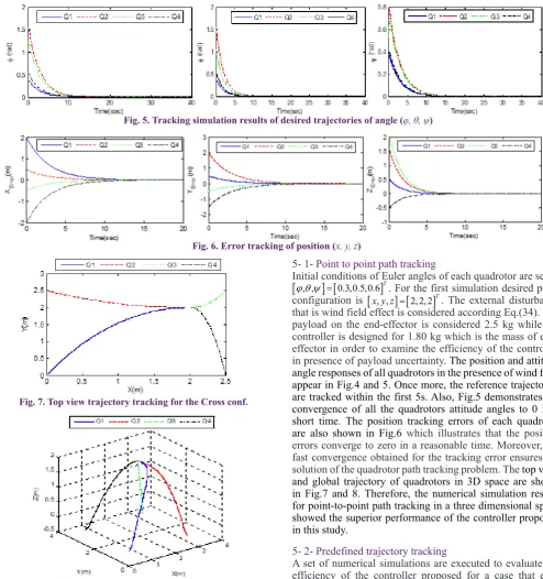
The position and attitude angle responses of the system in presence of wind field effect in predefined trajectory tracking are shown in Figs.9 and 10. The proposed controller stabilizes the attitude angle at 0 rad in a short time. It can be seen that the control inputs are smooth and free of any chattering. The tracking trajectory of all quadrotors appear in Fig.10. It is shown that even though the position and attitude of the quadrotors are affected by the abruptly changed reference Fig. 5. Tracking simulation results of desired trajectories of angle (φ, θ, ψ)

Fig. 6. Error tracking of position (x, y, z)

Fig. 7. Top view trajectory tracking for the Cross conf.

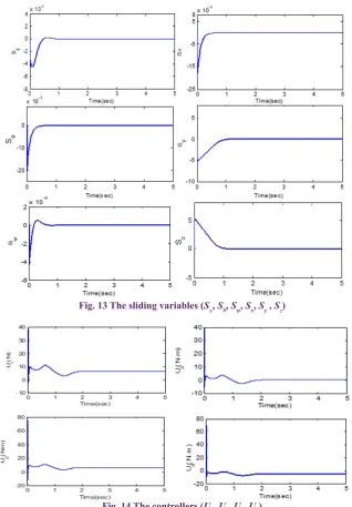
positions and angles, the controller is able to drive all these state variables back to the new reference position and angle within seconds which is a mandatory characteristic to control a system such as the quadcopter. The top view trajectory tracking and trajectory of all quadrotors in 3D space are shown in Fig.11 and 12. We see that the system performs well and tracks the desired trajectory in three-dimensions. Results

indicate that quadrotors lift up and down the object, and stable grasp has been achieved. Moreover, the aerodynamic forces and moments and air drag are taken into account in the controller design which demonstrate the robustness and effectiveness of the designed cooperative control scheme. The behavior of the sliding variables, shown in Fig.13, follows the expectations as all these variables converge to their sliding surfaces. Moreover, the position and velocity tracking errors of the system state variables are perfectly explained by the fluctuations of these sliding variables. Finally, Fig.14 shows the stability rotor speed response of a Quadrotor during hovering. The control inputs are smooth and the chattering phenomenon is decreased using the proposed controller. The amplitudes of the control inputs are also practically realizable and small. In a practical sense, the energy reduction enforces a longer autonomous flying period for the quadrotor which is still a major problem for this kind of mobile robots.

6- Conclusion and Future Works

In this paper, the problem of controlling multiple quadrotors that cooperatively manipulate and transport a payload in three dimensions was properly addressed. An optimal decentralized control algorithm based on second order sliding mode controller (SOSMC) approach using extended kalman-bucy filter (EKBF) as an observer has been proposed for a group of cooperative quadrotors. First, a model for a single quadrotor and then a team of quadrotors rigidly attached to a payload were developed. Individual robot control laws were introduced with respect to the payload to stabilize the payload along three-dimensional trajectories. This method offers an efficient and systematic procedure to solve a non-linear closed-loop optimal robust control problem. In order to validate the efficacy and optimality of the proposed method, simulation results were presented. Simulation results suggest that our method demonstrates better performance in the presence of external disturbances and parametric uncertainties such as wind field effects. Qualities of high accuracy, small position errors, minimum influence of the nonlinearities on the performance of cooperative UAVs, and versatility to a variety of maneuvers are other advantages of our proposed method. As a future work, the authors seek to develop a multi-Fig. 9. Tracking simulation results of desired trajectories of angle (ϕ, θ, ψ)

Fig. 10. Tracking simulation results of desired trajectories of position (x, y, z)

Fig. 11. Top view trajectory tracking for the Cross conf.

stage sliding controller to maintain the states at desired values while using the Load Sharing approach among multiple agents in order to improve design performance gained in this paper.

Reference

[1] M.H. Korayem, A. Zehfroosh, H. Tourajizadeh, S. Manteghi, Optimal Motion Planning of Non-linear Dynamic Systems in the Presence of Obstacles and Moving Boundaries Using SDRE: Application on CableSuspended Robot, Nonlinear Dyn, 76(2) (2014)1423-1441.

[2]  K. Das, R. Fierro, V. Kumar, J.P. Ostrowski, J.Spletzer, C.Taylor, A vision-based formation control framework, IEEE Transactions on Robotics and Automation, 18(5) (2002) 813-825.

[3] J. Sanchez, R. Fierro, Sliding mode control for robot formations, In: Proceedings of the 2003 IEEE International Symposium on Intelligent Control, Houston, USA, 2003.

[4] O.A.A. Orqueda, R. Fierro, Robust vision-based nonlinear formation control, In: Proceedings of the 2006 American Control Conference, Minneapolis, USA, 2006. [5] T.J. Tarn, A.K. Bejczy, X. Yun, Coordinated Control

of Two Robot Arms, In: Proceedingog 1986 IEEE International Conference Robotics and Automation , San Francisco, USA, 1986.

[6] S.C. LIU, D.L. Tan, G.J. Lui, Robust Leader-follower Formation Control of Mobile Robots Based on a Second Order Kinematics Model, Acta Automatica Sinica, 33(9) (2007) 947–955.

[7] R. Babaei, A.F. Ehyaei, A Novel UAV Cooperative Approach for Industrial Inspec on and Monitoring, In: Proceeding of 31st International Power System Conference (PSC), Tehran, Iran,2016.

[8] P. Cheng, J. Fink, S. Kim, V. Kumar, Cooperative towing with multiple robots, Algorithmic Foundation of Robotics VIII. Springer Tracts in Advanced Robotics, 57 ( 2008) 101-116.

Fig. 13 The sliding variables (Sφ, Sθ, Sψ, Sx, Sy , Sz)

[9] N. Michael, J. Fink, V. Kumar, Cooperative manipulation and transportation with aerial robots, Autonomous Robots , 30(1) (2011) 73-86.

[10] J. Fink, N. Michael, S. Kim, V. Kumar, Planning and

control for cooperative manipulation and transportation with aerial robots, Int. J. Rob. Res, 30(1) (2010) 324–334. [11]  M. Bernard, K. Kondak, I. Maza, A. Ollero, Autonomous

transportation and deployment with aerial robots for search and rescue missions, Journal of Field Robotics, 28(6) (2011) 914–931.

[12] G. Wang, X. Nian, H. Wang, Cooperative control of

discrete-time linear multi-agent systems with fixed information structure, J Control Theory , 10(3) (2012) 403–409.

[13] A.R. Patel, M.A. Patel, D.R. Vyas, Modeling and

analysis of quadrotor using sliding mode control, In: Proceeding of the 44th IEEE Southeastern Symp. on System Theory, Jacksonville , 2012.

[14] L. Besnard, Y.B. Shtessel, B. Landrum, Quadrotor

vehicle control via sliding mode controller driven by sliding mode disturbance observe , Journal of the Franklin Institute, 349 (2)(2012) 658-684.

[15] B. Sumantri, N. Uchiyama, S. Sano, Y. Kawabata,

Robust tracking control of a quad-rotor helicopter utilizing sliding mode control with a nonlinear sliding surface, J. System Design and Dynamics, 7(2)(2013) 226-241.

[16] B. Sumantri, N. Uchiyama, S. Sano, Least square

based sliding mode control for a quad-rotor helicopter, In: Proceeding of IEEE/SICE Int. Symp. on System Integration, Kobe ,2013.

[17] J.J. Xiong , E.H. Zheng, Position and attitude tracking control for a quadrotor UAV, ISA Transaction, 53(3) (2014) 725-731.

[18] R. Babaei, A. FEhyaei, Robust Control Design of

a quadrotor UA Based on Incremental Hierarchical Sliding Mode Approach, In: 25th Iranian Conference on Electrical Engineering (lCEE), Tehran, Iran, 2017.

[19] L. Derafa, A. Benallegue, L. Fridman, Super twisting

control algorithm for the attitude tracking of a four rotors UAV, Journal of the Franklin Institute , 349 (2) (2012) 685-699.

[20] L.L.Vegan, B.C.Toledo, and A.G.Loukianov, Robust

block second order sliding mode control for a quadrotor, Journal of the Franklin Institute , 349 (2) (2012) 719-739

[21] M. Bouchoucha, S. Seghour, M. Tadjine, Classical

and second order sliding mode control solution to an attitude stabilization of a four rotors helicopter: from theory to experiment , In: Proceedings of the 2011 IEEE international conference on mechatronics , Istanbul,

Turkey , 2011

[22] I. Eker, Second-order sliding mode control with

experimental application, ISA Transaction, 49(3) (2010) 394–405.

[23] S. Mondal, C. Mahanta, A fast converging robust

controller using adaptive second order sliding mode, ISA Transaction, 51 (6) (2012) 713–721.

[24] Z.Q. Guo, J.X. Xu, T.H. Lee, Design and implementation of a new sliding mode controller on an underactuated wheeled inverted pendulum, Journal of the Franklin Institute , 351(4) (2014) 2261–2282.

[25] L. Besnard, Y.B. Shtessel, B. Landrum , Quadrotor

vehicle control via sliding mode controller driven by sliding mode disturbance observer, Journal of the Franklin Institute, 349 (2) (2012) 658–84.

[26] C. Coza, C. Nicol, C.J.B. Macnab ,A. Ramirez-Serrano

, Adaptive fuzzy control for a quadrotor helicopter robust to wind buffeting, Journal of Intelligent and Fuzzy Systems , 22(5)(2011) 267–83.

[27] R. Babaie , A.F. Ehyaei, Robust optimal motion planning approach to cooperative grasping and transporting using multiple UAVs based on SDRE , Transaction of the Institute of Measurement and Control , 39(9)(2017)1391-1408.

[28] D. Mellinger, M. Shomin, N. Michael, V. Kumar ,

Cooperative Grasping and Transport Using Multiple quadrotors, Distributed Autonomous Robotic Systems. Springer Tracts in Advanced Robotics, 83( 2013) 545-558.

[29] M. Rhudy, Y. Gu, M.R. Napolitano, An Analytical

Approach for Comparing Linearization Methods in EKF and UKF, International Journal of Advanced Robotic Systems, 10 (208) (2013).

[30] M. Rhudy, Y. Gu , Understanding Nonlinear Kalman

Filters Part I: Selection of EKF or UKF, Interactive Robotics Letters, Link: http://www2.statler.wvu.edu/~irl/ page13.html, 2013.

[31] R. Babaie, A.F. Ehyaei, Robust Backstepping Control of a quadrotor UAV Using Extended Kalman Bucy Filter, International Journal of Mechatronics, Electrical and Computer Technology, 5(16) (2015) 2276- 2291.

[32] K. Runcharoo, V. Srichatrapimuk, Sliding Mode Control of quadrotor, In: Proceeding of International Conference of Technological Advances in Electrical, Electronics and Computer Engineering (TAEECE), Konya, 2013.

[33] L.Wang, C. He, P. Zhu, Adaptive Sliding Mode Control

for quadrotor Aerial Robot with Ι Type Configuration, International Journal of Automation and Control Engineering , 3(1) (2014) 20-26.

Pleasecitethisarticleusing:

R. Babaie and A. F. Ehyaei, Cooperative Control of Multiple quadrotors for Transporting a Common Payload, AUT J. Model. Simul., 50(2) (2018) 147-156.