Copyright 1999 Air & Waste Management Association
Application of the Shifting Method as a Technique to Correct for
the Background in Quantitative Analysis by Open-Path FTIR
Stefanie Giese-Bogdan
University of Michigan, School of Public Health, Ann Arbor, Michigan, and Gerhard Mercator Universität
-Gesamthochschule Duisburg, FB6 - Instrumental Analytical Chemistry
Steven P. Levine
University of Michigan, School of Public Health, Ann Arbor, Michigan
Karl Molt
Gerhard Mercator Universität - Gesamthochschule Duisburg, FB6 - Instrumental Analytical Chemistry
ABSTRACT
In open-path Fourier Transform Infrared spectroscopy, the generation of a suitable background single-beam spectrum is of major concern. The Shifting Method is a derivative-like approach to correct for the background without the need to actually measure a background spectrum using the sample single-beam spectrum. A thorough study of the Shifting Method was conducted. A set of guidelines was developed based on the results of artificial and closed cell data. These guidelines were applied to three different data sets, consisting of cell and open path data with multiple com-pounds, overlapping peaks, and high water vapor and aerosol levels.
INTRODUCTION
The technology of open-path Fourier Transform Infra-red spectroscopy (op-FTIR) has found a wide range of applications over the last years1 for such diverse appli-cations as outdoor and indoor analysis at industrial sites as well as in homes.1-9 FTIR instruments usually are single-beam instruments, which makes the sepa-rate acquisition of a background single-beam spectrum (SB-spectrum) necessary to obtain transmittance spec-tra. In op-FTIR setup, the acquisition of a background spectrum under the same conditions as the sample
IMPLICATIONS
Continuous air monitoring with open-path Fourier Trans-form Infrared spectroscopy can be perTrans-formed without the need to actually measure a background spectrum and with assurance that the baseline will be accurate.
spectrum, but without containing the analytes, is ex-perimentally difficult.
Over the years, multiple methods for correction of the background have been developed to overcome this problem.10,11 In general, one can try to record an analyte-free background spectrum by modifying the experimen-tal conditions under which the sample is taken. Another way is to manipulate the sample SB-spectrum itself to derive a suitable background spectrum. Methods that are based on obtaining an actual background SB-spectrum are called “Library,” “Short-path,” “Upwind/Sidewind,” and “Average Background.”10-12 Methods based on manipula-tion of the sample SB-spectrum include the methods of generating a synthetic background, “Backfitting” and “It-erative Adaptations.”13-16 For all methods listed, some gen-eral statements can be made:
• They are complicated and require a high degree of experience.
• None of them is valid for all applications of op-FTIR. (The applicability varies from situation to situation.)
• They are work- and time-intensive. • They are location- and time-dependent. • They have to be repeated frequently.
The Shifting Method for use in op-FTIR was first in-troduced in 1993.17 This method is a derivative-like ap-proach to correct for the background without the need to actually measure a background spectrum using the sample SB-spectrum. Therefore, there is no dependency on loca-tion and time, which can cause serious problems in quan-titative analysis of op-FTIR spectra.15
quantitative gas analysis with FTIR. It also proved to be better than first derivatives calculated with Savitzky-Golay filter functions.1 The conclusions drawn from this study were summarized as a set of guidelines as follows:
• A shift has to be an integer multiple of the digi-tal resolution in order to avoid numerical errors. • For spectra with a small amount of noise or sharp bands of large amplitudes, a shift of a few wavenumbers is sufficient. The broader the peak and the higher the noise level, the larger the required shift. Good results are achieved when shifting between half and the full Full-Width-at-Half-Height (FWHH) of the broadest band.
• When quantifying using only one peak, a lineshift due to lack of reproducibility of the wavenumber axis that is smaller than 10% of the FWHH will cause a deviation from the real concentration by not more than approxi-mately ±5%. This means that especially for sharp bands, a high degree of reproducibil-ity or, alternatively, a wavenumber correc-tion, is necessary.
• As is valid for most analytical methods and for the use of Classical Least Squares (CLS) analysis as a quantification tool, the con-centration of the reference spectrum should be in the same range as the concentration of the sample spectrum to avoid deviations from linearity.
This paper presents the application of the Shifting Method using these guidelines for data with overlapping peaks and field data containing methanol and ammonia, as well as spectra obtained under high water vapor and aerosol conditions.
MATHEMATICAL DESCRIPTION OF THE SHIFTING METHOD
One important condition for quantitative spectrometric analysis is a linear relationship between absorbance and concentration, as stated in Lambert-Beer’s law:
log
10 0I
I
= − ⋅ ⋅
ε
c d
(1)In the case of FTIR spectrometry, I is the single-beam sample and I0 the single-beam background spectrum.
One alternative to “ratioing” against a background spectrum is the calculation of first derivatives67,68 of the negative logarithm of the SB-spectrum.69 This leads to the single-beam derivative (SD) absorbance spec-trum, A’SB,
A
SBI
c d
I
'
(log
)'
' ( ˜ )
(log
)'
= −
10=
ε υ
⋅ ⋅ −
10 0 (2)Eq 2 shows that for A’SB, there exists (for a given pathlength d) a linear relationship with the concentra-tion if (log10I0)’ remains constant. This is equivalent to the demand that the ratio between the slope and the abso-lute value of I0remains constant at the wavenumber (~)υ , at which the following is measured:
− = − = −
⋅ =
(log )' log ( ˜ )
˜
' ( ˜ )
( ˜ ) ln .
10 0
10 0 0
0 10
I d I
d
I
I const
υ υ
υ
υ (3)
This condition is practically always fulfilled, because the numerical value of I0'( ~)ν is negligible compared with the one for I0(
~)
ν . In practice, this results in a baseline around zero for derivative spectra. Hence, the usual numerical methods of linear algebra can be applied to the multivariate analysis of SD-absor-bance spectra.
The Shifting Method uses the original SB-spectrum shifted by ∆υ~ for ratioing
A I
I
SB
∆
∆
( ˜ ) log ( ˜ ) ( ˜ ˜ )
υ υ
υ υ
= −
+ 10
(4)
A
SB∆ is the shift ratioed absorbance spectrum (SR-absor-bance spectrum), if ∆υ~ is small compared with the FWHH, the following approximation holds:A
SB∆≈
A
'
SB⋅
∆
υ
˜
(5)Eq 5 shows that for SR-absorbance spectra, the same con-ditions for the applicability of linear multivariate analy-sis hold as for SD-absorbance spectra. Further, the ampli-tude of SR-absorbance spectra is proportional to the in-crement used for shifting.
When applying the Shifting Method, each single-beam sample spectrum has to undergo the process math-ematically described by eq 4.
QUANTITATIVE ANALYSIS
Quantitative analysis was performed by means of CLS analysis.18 In this method, a spectrum with a known con-centration (reference spectrum) is fitted to the spectrum of an unknown (sample spectrum).
To be able to apply Lambert-Beer’s law for quantifi-cation, the absorbance of each individual compound in a mixture cannot be affected by the presence of other compounds.19
A k A e
A k A e
A k A e
A k A e
s j j r j m s j j r j m i s ij ij r j m i n s nj nj r j m n
1 1 1
1
1
2 2 2
1 2 1 1 = ⋅ + = ⋅ + = ⋅ + = ⋅ + = = = =
∑
∑
∑
∑
... ... (6)where As = absorbance in sample; Ar = absorbance in refer-ence; i = wavenumber (total of n wavenumbers); j = com-ponent (total of m comcom-ponents); cs = sample concentra-tion; cr = reference concentration; and k c
c s r
= = concentra-tion ratio. For computaconcentra-tional purposes, the use of a ma-trix representation for eq 6 is easier
A
A
A
k
k
k
k
k
k
k
k
A
A
e
e
e
s s n s mn n nm
r m r n 1 2
11 12 1
21 22 1 2 1 1 2
M
K
M
M
M
K
M
M
=
×
+
(7)This can be written as
A
(sn )K
( )A
( )e
( )n m m
r
n
×1
=
×⋅
×1+
×1 (8)where the bold print represents the respective matrix. Different models have been developed to take into account the underlying baseline.20 The quantification soft-ware used in this study presumed that the baseline of sample and reference spectra was linear over each peak (ETG Continuous Monitor Analysis Software). As a con-sequence, different equations have to be set up for every single peak. The concentration of a compound j is pre-sumed to be constant over a peak p.
The absorbance of a sample s at a wavenumber i for a peak p can then be written as an expansion of eq 6
A
ipa
b
k A
e
s
p p i jp ijp
r ip j m
=
+
+
+
=∑
λ
1 (9)with
a
p+ λ
b
p i being the linear equation for the baseline (9a), andA
ips= absorbance of sample at wavenumber i
a n d p e a k p;
A
ip
r = a b s o r b a n c e o f r e f e r e n c e a t
wavenumber i and peak p; i = wavenumber i = 1 ... n; j
= c o m p o u n d j = 1 . . . m ; a n d ei p = r e s i d u a l a t wavenumber i of peak p.
For computing purposes, the following matrix repre-sentation for the least squares method for a linear baseline over a peak (eq 9) was used
A A
A
A A A
A A A
A A A
a b k k k e e s s n s r r m r r r m r n n r n r nm r m 1 2
1 11 12 1
2 21 22 2
1 2 1 2 1 2 1 1 1 M K K
M M M M M
K M M = × + λ λ
λ een
(10) This can be written as
As
(n x 1) = U[n x (m+2)]S[(m+2) x 1] + e(n x 1) (11)
where the bold print represents the respective matrix. The ratio of cs
j / c r
j = kj and the slope and intercept of the linear baseline (Vector S) was calculated separately for each peak, using the CLS analysis method so that the sum of squares of the error was minimized. The different k
values for each compound were pooled. Different weight-ing factors were then applied to calculate a final kj and, thus, concentration
c
js.20To be able to use mathematical tools such as CLS analysis for quantification of spectra generated using the Shifting Method, the single-beam reference spectrum has to be treated the exact same way, using the identical ∆υ~ (eq 5) for the reference and sample spectrum.
EXPERIMENTAL DATA AND METHODS
Three data sets were used: closed cell data, open-path data from a wastewater treatment plant, and open-path data with high water vapor and aerosol concentration.
Closed Cell Data
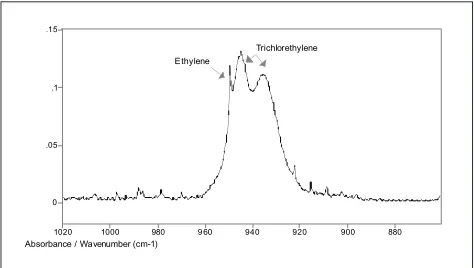
Spectra of compounds with overlapping peaks were gen-erated in a benchtop FTIR (Perkin Elmer 2000) equipped with a 10-cm cell and a mercury-cadmium-telluride (MCT) detector. Mixtures of ethylene and trichloroethylene were
0 .05 .1 .15
1020 1000 980 9 60 940 920 900 880 Absorbance / Wavenumber (cm-1)
Ethylene
[image:3.612.317.554.563.697.2]Trichlorethylene
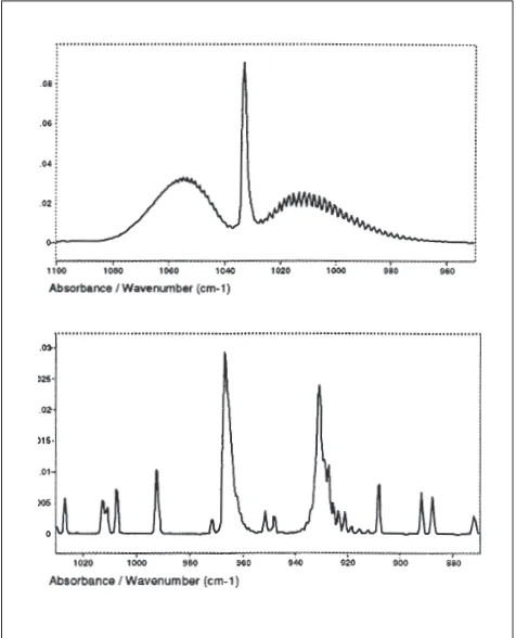
used for this study. The two compounds show one over-lapping feature in the fingerprint region (ethylene, CH2 -wagging at 949 cm-1 and trichloroethylene, CCl stretch band at 912–966 cm-1).
Figure 1 shows an absorbance spectrum of a mixture with 400 ppm*m ethylene and 1,600 ppm*m trichloroet-hylene. The overlapping feature was used for CLS analy-sis (wavenumber range for quantification approximately 900–980 cm-1—adjusted depending on the shift). Since a cell was used, a true background spectrum could be used to compare the results of the Shifting Method with those of the conventional method using a clean background SB-spectrum to calculate an absorbance spectrum.
The mixtures were made by mixing trichloroethyl-ene and ethyltrichloroethyl-ene from certified gas standards in various ratios, without using additional dilution gas. Three mix-tures were prepared:
• Mixture 1: 1,600 ppm*m ethylene, 400 ppm*m trichloroethylene
• Mixture 2: 1,000 ppm*m ethylene, 1,000 ppm*m trichloroethylene
• Mixture 3: 400 ppm*m ethylene, 1,600 ppm*m trichloroethylene
Reference spectra were generated under the same ex-perimental conditions for the single compounds; the ref-erence concentration for each compound was 1,000
ppm*m. In the wavenumber range of interest, water was not an interference. The use of certified cylinders with the analytes diluted in nitrogen made adding a water spec-trum to the quantitative analysis unnecessary.
Open-Path Data from a Wastewater Treatment Plant
This data set was generated at a wastewater treatment plant of a petrochemical facility in Germany.21 This facility treated industrial and sanitary sewage from the petrochemical facility. The wastewater treatment plant consisted of two basins of 10 m × 20 m and one sew-age drainsew-age.
The instrument used for this study was an op-FTIR (ETG Co.). It was equipped with a MCT detector that was cooled with a Sterling engine. The setup was monostatic, with a total pathlength of 196 m and an optical resolu-tion of 1.0 cm-1 (digital resolution 0.5 cm-1). The instrument was installed about 2 m above the water level in the basins. Compounds analyzed in this study were methanol and ammonia. Figure 2 shows reference absorbance spec-tra of these two compounds in the regions that were used for quantification. The concentration-pathlength prod-uct peak intensities of the sample spectra were in the same range as those of the reference spectra. For the quantita-tive analysis by means of CLS, the fingerprint regions of both compounds were used. The region used for analysis was adjusted according to the amount of shift and was in the range of 880 to 1,200 cm-1.
Open-Path Data with High Water Vapor and Aerosol Concentration
This data set was part of a series of experiments to study the influence of humidity and water aerosols on limits of detection and noise levels in op-FTIR.22
The experiments took place in a chamber that was 0.85-m wide, 1.18-m long, and 1.53-m high. The cham-ber was equipped with a shower to generate extremely high water vapor concentration and water aerosol condi-tions. The FTIR beam crossed the chamber at a height of 110 cm from the chamber floor. An aqueous solution of chloroform was injected into the water stream prior to entering the chamber. The data set was used in this study because it represented the worst case scenario for water vapor concentration.
The instrument used was an op-FTIR (Nicolet Instru-ment Corp., Madison, WI), with a liquid-nitrogen-cooled MCT detector. The setup was bistatic with a pathlength of 1 m. The optical resolution was set to 2 cm-1.
[image:4.612.58.296.425.719.2]The reference spectrum was obtained with a Nicolet 550 bench FTIR (Nicolet Instrument Corp., Madison, WI) fitted with a 4.8 m gas cell and an MCT detector. The reference absorbance spectrum
of chloroform showed a peak at 772 cm-1 that was used for quantitative analysis (Figure 3).
RESULTS AND DISCUSSION Closed Cell Data
Applications of the Shifting Method to this data using the guidelines developed was expected to give good results, since the instrument noise level was low and spectral purity was high in this data set. The data set was generated using a closed sample cell, which made obtaining a background SB-spectrum possible. Thus, the results of the Shifting Method could be compared directly with those of the conventional method.
Besides those two methods, the method of first de-rivatives was used without (Point difference) and with fil-ter functions affil-ter Savitzky-Golay.25 The Shifting Method calculates differences in ordinate without a smoothing function. Savitzky-Golay filter functions are moving filter functions, corresponding to a least squares fit in
a specified window of data points. The degree of smooth-ing is determined by the order of the polynomial that is fitted and the number of data points over which the fit is calculated. A polynomial of the second order was used for this study with two different numbers of points, 5 and 15. The method of first derivatives was applied to the single-beam sample and single-single-beam reference spectra (eq 2).
Based on results obtained on artificial and laboratory data,1 all four methods were expected to be suitable for this data set.
For the Shifting Method, three different shifts of 1, 3, and 10 cm-1 were selected. Using the guidelines, for ethyl-ene, a shift of 1 cm-1 to 3 cm-1 was expected to give the best results. For the same reasons, for trichloroethylene, a shift of 1 cm-1 was expected to give results that are not as good as they would be for larger shifts.
The Shifting Method was expected to detect ethyl-ene without large differences from the true concentra-tion, since it was a sharp peak without extensive fine struc-ture. For trichloroethylene, larger necessary shifts than for ethylene were expected, since the spectral feature of trichloroethylene (FWHH 20.7 cm-1) was broad compared with ethylene (FWHH 1.2 cm-1).
Since the noise level in these spectra was low, the difference between smoothed and unsmoothed first de-rivatives was expected to be small. Table 1 shows the re-sults for the different mixtures and methods. The con-centrations are given in ppm*m. The standard deviation σ is an estimate of the analytical error.
The results in Table 1 show that the method of first derivatives without smoothing (point difference) gave concentration results that differed significantly from the results of the conventional method. The dif-ferences were between 17.4% and 24.5% for trichloro-ethylene. At the 400 ppm*m level, point difference 0
.05 .1 .15 .2 .25
860 840 820 800 780 760 740 7 20 700 680
[image:5.612.55.293.59.208.2]Absorbance / Wavenumber (cm-1)
Figure 3. Absorbance reference spectrum of chloroform. Concentration 96 ppm*m. The spectrum was generated in a cell with a benchtop FTIR with a resolution of 2 cm-1.
Table 1. Results for the quantitative analysis of three mixtures of ethylene and trichloroethylene (TCE) with the Shifting Method (three different shifts), first derivatives with and without smoothing and the conventional method. Concentrations are given in ppm*m. The standard deviation σ is the standard deviation for the fit of the CLS analysis.
Mixture Shift TCE σ Ethylene σ TCE σ Ethylene σ
[cm-1] [ppm*m] [ppm*m] [ppm*m] [ppm*m]
1 1 1,541 7.7 419 1.9 Point difference 1,309 21.7 414 5 3 1,561 2.5 416 1.1 Sav.-Gol 5 point 1,432 16.3 416 3.3 10 1,551 1.8 405 1.5 Sav.-Gol 15 point 1,557 4.7 420 0.9 Actual Conc. 1,600 400 Convent. method 1,585 0.4 414 0.6
2 1 978 7.3 1,011 1.9 Point difference 760 19.7 1,010 4.3 3 995 2.5 1,006 1.3 Sav.-Gol 5 point 876 15.3 1,011 3.2 10 983 1.8 995 1.3 Sav.-Gol 15 point 993 4.3 1,011 1.1 Actual Conc. 1,000 1,000 Convent. method 1,007 0.4 1,005 0.9
[image:5.612.54.553.551.742.2]could not detect trichloroethylene at all. The tions for ethylene were smaller, the maximum devia-tion 1%.
Smoothing of the data with the 5-point Savitzky-Golay function improved the results for trichloroethyl-ene. The difference between the results obtained using the conventional method was 10.4% for mixture 1, 13% for mixture 2, and 29.4% for mixture 3. Stronger smooth-ing (15-point Savitzky-Golay) greatly improved the re-sults, the largest deviation from the real concentration being 2%. For ethylene, smoothing of the data did not significantly improve the results. The deviations were still about only 1%.
The Shifting Method gave good results for both com-pounds. A shift of 1 cm-1 gave results that showed a maxi-mum deviation of 2.9% for trichloroethylene. The results for ethylene were within 1.2% of the conventional method. The best results for ethylene were achieved with a shift of 3 cm-1, the maximum difference to the conven-tional method was 0.5%. Ethylene was expected to be best analyzed at small shifts because the spectral feature of eth-ylene is a strong sharp peak. The peak-to-peak amplitude of the signal at 3 cm-1 is larger than at 1 cm-1, which may lead to better results for the larger shift.
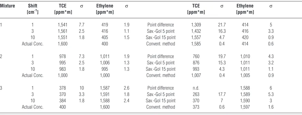
For trichloroethylene, a shift of 3 cm-1 gave the best results; the maximum difference to the conventional method was 1.5% (for the lowest concentration). The dif-ference was 1.2% for mixture 2, and 0.6% for mixture 3. A shift of 10 cm-1 resulted in large differences from the calculated value for both ethylene and trichloroethylene. A shift of 10 cm-1 was expected to give better results for trichloroethylene because 10 cm-1 was equal to half of the FWHH of the overall peak. Figure 4 shows the absorbance spectrum of trichloroethylene for a shift of 3 cm-1 and for a shift of 10 cm-1. Since the peak is a doublett, the com-posing bands of which have a considerably smaller FWHH, the shifting should be adapted to the smaller FWHH. This can be seen in Figure 4.
Another reason could be that the narrower ethylene peak could be determined more accurately at smaller shifts and, therefore, made the quantification of trichloroeth-ylene more accurate. A comparison of the spectra in Fig-ure 5 shows that the ethylene peak is much more pro-nounced at a shift of 3 cm-1 than at 10 cm-1.
Although the noise level was small, the method of point differences and weak 5-point Savitzky-Golay smoothing showed large differences to the conventional method (about 20%). Both methods were not accurate for this data set. The 15-point Savitzky-Golay method was accurate for this data set. The results showed differences of about 2% from the conventional method.
[image:6.612.321.558.56.355.2]The Shifting Method proved to be accurate for both compounds in all mixtures and for all shifts. The best
Figure 4. Absorbance spectra of trichloroethylene 1,000 ppm*m, generated with the Shifting Method using a shift of 3 cm-1 (left) and
with a shift of 10 cm-1 (right).
[image:6.612.321.559.409.704.2]results were achieved with a shift of 3 cm-1. The differ-ences from the conventional method were comparable for trichloroethylene and ethylene (max 3%).
Open-Path Data: Wastewater Treatment Plant The spectra were analyzed using two methods to gener-ate absorbance spectra: the conventional method and the Shifting Method. In order to generate absorbance spectra with the conventional method, a synthetic background was calculated. Figure 6 shows a single-beam sample spectrum with the synthetic single-beam background spectrum. For illustration purposes, a slight offset in the y-axis was in-troduced to show both curves in one figure. Figure 7 shows the resulting absorbance spectrum in that region.
For the Shifting Method, three different shifts were tested. Three shifts of 3 cm-1, 5 cm-1, and 10 cm-1 were tested. The shifts of 3 cm-1 and 5 cm-1 were expected to give very similar results because they were about equal to the FWHH of the peaks. The shifts of 10 cm-1 were expected to give results that were low compared with
those from smaller shifts, because the peaks would be totally resolved for a shift of 10 cm-1 and the effect of noise would increase.
Figure 8 shows a diagram of the results for methanol and ammonia. For methanol, the results were best for a shift of 5 cm-1. At a shift of 3 cm-1, two samples were be-low the 3σ minimum detection limit. A shift of 5 cm-1 improved the minimum detection limit because the en-hancement of the signal was slightly stronger than for a shift of 3 cm-1. A shift of 10 cm-1 did not improve the results because the peak was going through an inflection point. This produced a negative effect on the concentra-tion analysis, the minimum detecconcentra-tion limit was higher than for a shift of 5 cm-1, and four samples were below the minimum detection limit (11 min, 13 min, 15 min, and 16 min).
For ammonia, all shifts gave results that clearly showed the same variation of concentration with time. A shift of 5 cm-1 gave results that were for all samples slightly higher than the results of the conventional method. A shift of 3 cm-1 gave results that were very close to those of
12 14 16 18 20 22 24
1100 1050 1000 950 900 850
[image:7.612.54.291.345.493.2]Arbitrary Y / Wavenumber (cm-1)
Figure 6. Single-beam sample spectrum obtained at the wastewater treatment plant (bottom curve) and synthetic background spectrum (top curve). For demonstration purposes, an offset in the y-axis was introduced.
0 .1 .2 .3
[image:7.612.318.555.354.689.2]1150 1100 1 050 1000 950 900 850 800 Absorbance / Wavenumber (cm-1)
Figure 7. Background ratioed absorbance sample spectrum of the single-beam sample spectrum obtained at the wastewater treatment plant and displayed in Figure 6, generated with the synthetic background spectrum as displayed in Figure 6.
0 0.1 0.2 0.3 0.4 0.5 0.6
0 2 4 6 8 10 12 14 16
Time [min] Conc.
[ppm]
Convent. Method Shifting 3 cm-1
Shifting 5 cm-1 Shifting 10 cm-1
0.03 0.04 0.05 0.06 0.07
0 2 4 6 8 10 12 14 16
Time [min] Conc.
[ppm]
Convent. Method Shifting 3 cm-1
Shiftng 5 cm-1 Shifting 10 cm-1
Figure 8. Data from the wastewater treatment plant. Concentration results [ppm*m] for methanol (A) and ammonia (B) using the conventional method and the Shifting Method with three different shifts (3 cm-1, 5 cm-1, and 10 cm-1). Concentration analysis results are shown
for samples taken at various times [min].
a
b Convent. Method Shifting 3 cm-1
Shifting 5 cm-1 Shifting 10 cm-1
[min]
[image:7.612.54.292.546.697.2]the conventional method; only for three samples (11, 13, and 16 min) were the results higher. A shift of 10 cm-1 gave results that were for all samples slightly lower than those from the conventional method.
The Shifting Method proved to be suitable for this application of op-FTIR. A clearer difference between the results of different shifts had been expected. One reason for this not having occurred was that the concentration analysis was based on two peaks. Effects due to shifts that are better for one of the peaks may have been compen-sated for by contrary effects on the second peak due to the different FWHH of the two peaks.
The various shifts showed that for a peak with a small FWHH, such as the methanol peak, a shift of 5 cm-1 was sufficient, whereas a large shift degraded the detection limit and, therefore, worsened the results.
The Shifting Method proved to be applicable with one shift (5 cm-1) for two different compounds. The de-viations from the conventional method for that shift were between 20 and 30%. Deviations in that range are accept-able in applications for environmental and industrial health.23,24 A word of caution is needed at this point about the concentration analysis of the conventional method. Since the collection of a true background spectrum was not possible, a synthetic background had to be used. The use of such a background can introduce errors in the quan-titative analysis. Therefore, the true concentrations are not known. The Shifting Method could only be compared with the conventional method as a widely used back-ground correction method.
Open-Path Data: High Water Vapor and Aerosol Concentration
[image:8.612.320.559.359.507.2]As shown, the Shifting Method gave good results com-pared with the conventional method, when the environ-mental parameters were controlled or not too extreme. Since water vapor is one of the most critical factors influ-encing FTIR spectra, the Shifting Method was tested with a data set with high water vapor concentrations.
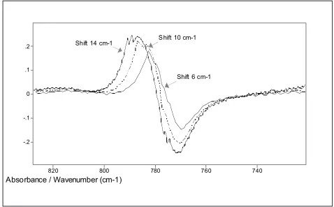
Figure 3 shows the reference spectrum of chloroform, the selected peak at 772 cm-1 had a FWHH of 14 cm-1. Applying the guidelines developed for the amount of shift necessary led to the assumption that a shift of 14 cm-1 would give the best results. A shift larger than 14 cm-1 would not result in a further improvement of the signal, since the maximum enhancement possible is reached when shifting is equal to the FWHH of a peak.
In addition to a shift of 14 cm-1, shifts of 6 cm-1 and 10 cm-1 were chosen. The results for the smaller shift of 6 cm-1 were expected to be low compared with those for a shift of 10 cm-1. The results for a shift of 10 cm-1 were expected to be low compared with those for a shift of 14 cm-1, since the FWHH of the selected peak was 14 cm-1.
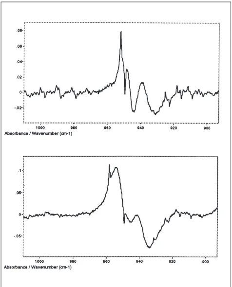
Figure 9 shows the resulting spectral features when applying the different shifts to the chloroform reference spectrum. A shift of 14 cm-1 resulted in the most enhanced feature with the highest degree of fine structure. A shift of 6 cm-1 resulted in the least enhanced spectral feature with no fine structure visible.
For the conventional method, a SB-spectrum obtained at the beginning of the experiment, before chloroform had been introduced, was used as a background. Figure 10 shows an example of the resulting absorbance sample spectra in the region of interest.
During the experiment, the intensity and, in some regions, the shape of the single-beam spectra changed. Reasons for this might be stability of the instrument as well as reasons due to the aerosol concentrations that may lead to scattering of the IR beam. (They were investigated in another part of the study of this data set.22) This can be seen in Figure 11, in which the single-beam spectra of four samples taken at different times during the experi-ment are shown.
Before calculating the absorbance spectra, an adjust-ment had to be made for the different energy levels in
Figure 9. Absorbance reference spectra of chloroform (96 ppm*m) generated with the Shifting Method applying a shift of 6 cm-1, 10 cm-1,
and 14 cm-1. The single-beam sample spectrum was generated in a
cell with a benchtop FTIR with a resolution of 2 cm-1.
-.2 -.1 0 .1 .2
820 800 780 760 740
Absorbance / Wavenumber (cm-1)
Shift 14 cm-1 S hift 10 cm-1
Shift 6 cm-1
.1 .12 .14 .16 .18 .2 .22 .24
8 20 800 780 760 740 720
Absorbance / Wavenumber (cm-1)
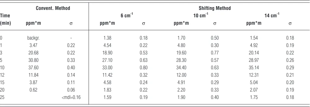
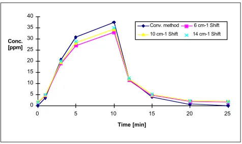
[image:8.612.322.558.563.710.2]sample and background SB-spectrum. Despite this adjust-ment, the resulting spectra showed baseline fluctuations, as can be seen in Figure 10, which showed that there were changes in the baseline in the course of the experiment. Table 2 shows the results of the quantitative analysis by means of CLS for the conventional method and the Shifting Method with three different shifts—6 cm-1, 10 cm-1, and 14 cm-1. The conventional method, as well as the Shifting Method, for all three shifts showed the same changes of the concentration with duration of the ex-periment as shown in Figure 12. All showed a rise in the concentration up to the highest concentration after 10 min. After 10 min, the injection of chloroform was stopped and the concentration decreased.
The standard deviations for the CLS analysis were good for all samples and all shifts (between 1 and 15%). The concentration results of a shift of 6 cm-1 showed larger discrepancies than those of the conventional method (12% for samples at 5 and 10 min). They improved with larger shifts (8% for samples at 5 and 10 min at a shift of 10 cm-1), which can be explained by the better enhance-ment of the signal. As was expected, a shift of 14 cm-1
showed concentrations and standard deviations of the least squares analysis of the spectra generated using the Shifting Method that were similar to those of the con-ventional method. The deviation in concentration be-tween the Shifting Method and the conventional method for samples at 5 min, as well as for samples at 10 min, was 6% for this shift.
The results of the Shifting Method for the high con-centration samples at 3, 5, 10, and 12 min were up to 6% lower than those of the conventional method. The re-sults for the lower concentration samples (1, 15, 20, and 25 min) were higher (up to 40%) for the Shifting Method than those for the conventional method. After 25 min, the conventional method was not able to detect any roform, whereas the Shifting Method still detected chlo-roform at levels between 1.6–1.9 ppm*m.
Since the real concentrations of the samples were unknown, a correct analysis could not be made. The Shift-ing Method could only be evaluated against the conven-tional method.
The absorbance spectra of the conventional method showed baseline fluctuations and were not generated by use of a “perfect” background. The SB-spectrum at the beginning of the experiment (0 min) was used as a back-ground SB-spectrum. The analysis of this spectrum with the Shifting Method showed that chloroform was already present at that time. The analyte-free spectrum was ap-parently contaminated with chloroform because the chamber could not be completely purged from earlier experiments. Thus, some chloroform was likely to have been left in the chamber air at the start of the next ex-periment. Since these effects may have influenced the concentration analysis, the results obtained using the conventional method were adjusted accordingly.
The Shifting Method proved to be applicable to this data set obtained under extremely high water vapor 0
1 2 3 4
4000 3500 3000 2500 2 000 1500 1 000 500
Arbitrary SB / Wavenumber (cm-1)
1min 20min 12min
[image:9.612.54.293.59.194.2]5min
[image:9.612.54.554.572.745.2]Figure 11. Single-beam sample spectra after 1 min, 5 min, 12 min, and 20 min duration of the experiment. There was no offset introduced to the spectra; the offset was measured as displayed.
Table 2. Open-path Data—high water vapor concentration, results of concentration analysis during the course of the experiment (time in min) with conventional and Shifting Method (6 cm-1, 10 cm-1, and 14 cm-1 shift). The standard deviation is the deviation in the least squares analysis.
Convent. Method Shifting Method
Time 6 cm-1 10 cm-1 14 cm-1
(min) ppm*m σ ppm*m σ ppm*m σ ppm*m σ
0 backgr. - 1.38 0.18 1.70 0.50 1.54 0.18
1 3.47 0.22 4.54 0.22 4.80 0.30 4.92 0.19
3 20.68 0.22 18.90 0.53 19.60 0.77 20.14 0.22
5 30.80 0.33 27.10 0.63 28.30 0.57 28.97 0.26
10 37.60 0.40 33.00 0.80 34.40 0.63 35.14 0.29
12 11.84 0.14 11.42 0.32 12.00 0.33 12.31 0.21
15 3.87 0.11 4.58 0.24 4.91 0.29 5.04 0.20
20 0.62 0.06 1.83 0.22 2.20 0.33 2.07 0.19
conditions. A shift equal to the FWHH of the chloroform peak at 780 cm-1 again gave the best results, as expected. However, smaller shifts up to a shift of half of the FWHH deviated only up to 7% from those results of a shift of 14 cm-1.
CONCLUSION
The studies presented were one part of an extensive study of the Shifting Method.1 The first two parts consisted of tests of the Shifting Method on artificial and laboratory data with single features. These tests led to the conclu-sion that the Shifting Method is a very useful tool for quantitative analysis of op-FTIR data. Evaluation under actual field use conditions with multiple compounds with overlapping peaks and under extreme high water vapor and aerosol concentrations showed that the guidelines developed on artificial and laboratory data proved cor-rect and applicable.
Good results were achieved when shifting between 0.5 and 1.0 of the FWHH of the spectral feature of inter-est. Best results were achieved when shifting equal to the FWHH of the spectral feature of interest. That was par-ticularly important for broad features (like those of chlo-roform). For spectral features with fine structure (like for trichloroethylene), smaller shifts led to better results be-cause the fine structure is lost when shifting equal to the FWHH of the broad underlying feature.
After testing the Shifting Method on artificial, closed cell and op-FTIR data, the conclusion can be drawn that the Shifting Method can be used to calculate absorbance spectra, without the need for recording a separate single-beam background spectrum.
The Shifting Method proved to be a fast and easy method to generate a derivative-like absorbance spec-trum. Once the optimal shift for a spectral feature is de-termined, the sample spectra can be processed without error caused by recording background spectra or check-ing the validity of existcheck-ing background spectra. The guide-lines presented help to find the optimal shift.
Depending on the complexity of the spectrum, the use of more than one shift may be necessary to achieve best results for the compounds present. However, accu-rate results are obtainable with a trivial increase in com-puting times.
If the application calls for long-term measurements of the same compounds, the Shifting Method provides accu-rate results, even if the spectrum is complex. In long-term measurements, instrumental imperfections as well as envi-ronmental changes can require a frequent generation of a background spectrum when using the conventional method. Since the Shifting Method is not influenced by these factors, it is superior to other background generation methods in long-term measurements.
The same can be said for continuous monitoring, such as alarm systems. In those cases, the detection of environmental and instrumental changes often is dif-ficult, as is accounting for these changes. This can lead to baseline fluctuations resulting in false positive or negative detection.20 The Shifting Method automati-cally accounts for these effects and, therefore, can give more reliable results.
The resulting baseline in the absorbance spectra generated with the Shifting Method is always close to zero. In addition, the Shifting Method makes the ac-curate determination of the location of a peak easy. Because of these effects, the Shifting Method is a use-ful tool to locate and identify unexpected compounds. The flat baseline also opens the way to computing strat-egies, such as iterative techniques to identify unex-pected compounds automatically. This will be a focus of future work on the Shifting Method.
Another focus will be the application of the Shift-ing Method to tomographic FTIR data. UsShift-ing op-FTIR for tomography requires the generation of mul-tiple background spectra for each set of scans. The Shifting Method may be one way to make the tomo-graphic op-FTIR techniques applicable to actual envi-ronmental field use applications.
ACKNOWLEDGMENTS
The authors would like to thank William McClenny, U.S. Environmental Protection Agency, for his financial sup-port and program management through Cooperative Agreement No. 822840; Dale Bacon at 3M Co. for the opportunity to generate data in his laboratory and for his technical mentorship; and Professor Michael Yost, University of Washington, Seattle, and Professor Konradin Weber, Fachhochschule Düsseldorf, for shar-ing vital and difficult to obtain data. They would also like to express their sincere thanks to George Russwurm, ManTech Inc., for his mentorship and friendship throughout this study.
0 5 10 15 20 25 30 35 40
0 5 10 15 20 25
Time [min] Conc.
[ppm]
[image:10.612.58.296.56.198.2]Conv. method 6 cm-1 Shift 10 cm-1 Shift 14 cm-1 Shift
REFERENCES
1. Giese-Bogdan, S. Optimization of Background Spectral Acquisition for Open Path Fourier Transform Infrared Spectroscopic Determina-tion of the ConcentraDetermina-tion of Gas and Vapor Contaminants in Ambi-ent Air. Ph.D. Dissertation, Gerhard Mercator University Duisburg (FRG), 1996.
2. Russwurm, G.M. The Use of Long Path FTIR Spectroscopy at the French Limited Superfund Site. In Proceedings of the 1993 U.S. EPA/A&WMA International Symposium on Field Screening Methods for Hazardous Waste
and Toxic Chemicals; Las Vegas, NV, February 1993.
3. Kagann, R.H.; Jolley, J.G.; Shoop, D.S.; Hankins, M.R.; Jackson, J.M. Open-path FTIR Measurements of Spatial Distributions of Chemical Emissions at Treatment, Storage and Disposal Facilities. Presented at the 86th Annual Meeting of the Air & Waste Management
Associa-tion (A&WMA), Denver, CO, 1993.
4. Haus, R.; Kaeding, H.; Leipnitz, W.; Bautzer, W. Open-path and Ex-tractive FTIS Measurements to Study Compost Emissions. In
Proceed-ings of the EUROPTO ’95, Munich, Germany, 1995.
5. Lamp, T.; Weber, K.; Weidemann, J.; vanHaren, G. Application of FTIR Spectroscopy to Open-path Measurements at Industrial Sites in Ger-many. In Proceedings of the A&WMA Specialty Conference on Optical Sensing for Environmental and Process Monitoring; A&WMA: Pittsburgh, PA, 1994.
6. Herget, W.F.; Levine, S.P. “Preliminary test of FTIR spectroscopy for monitoring semi-conductor process gas emissions,” Appl. Ind. Hyg.
1986, 2, 110.
7. Haus, R.; Schaefer, K.; Hughes, J.; Heland, J.; Bautzer, W. FTIS Remote Sensing of Smoke Stack and Test Flare Emissions. Presented at EUROPTO ’95, Munich, Germany, 1995.
8. Ying, L.S.; Levine, S.P.; Strang, C.R.; Herget, W.F. “FTIR spectroscopy for monitoring airborne gases and vapors of industrial hygiene con-cern,” Amer. Ind. Hyg. Assoc. J. 1989, 30, 354.
9. Zwicker, J.O.; Vaughan, W.M.; Dunaway, R.H. Open-path FTIR Measure-ments of Carpet/Water Sealant Emissions to Determine Indoor Air Qual-ity. In Proceedings of the A&WMA Specialty Conference on Optical Sensing for Environmental Monitoring; A&WMA: Pittsburgh, PA, 1993; SP-89. 10. Russwurm, G.M.; Childers, J.W. FT-IR Open-path Monitoring Guidance
Document, Second Edition; ManTech Environmental Technology, Inc.:
Research Triangle Park, NC, 1995; TR-4423-96-01.
11. Russwurm, G.M. Operational Considerations for the Use of FT-IR Open-path Techniques under Field Conditions. In Proceedings of EPA/ A&WMA Int. Symp. of Measurements of Toxic and Related Air Pollutants; A&WMA: Pittsburgh, PA, 1992; 579, VIP25.
12. Hunt, R.N.; Fuchs, P.A. Applications in Continuous Monitoring of Atmospheric Pollutants by Remote Sensing. In Proceedings of the A&WMA Specialty Conference on Optical Sensing for Environmental and Process Monitoring; A&WMA: Pittsburgh, PA, 1992; SP-81.
13. Simonds, M.A. Evaluation of the Role of Fixed Beam Open-Path Fourier Transform Infrared Spectroscopy in Air Monitoring Strategies, Ph.D. Dis-sertation, University of Michigan, School of Public Health, 1993. 14. Giese-Bogdan, S.; Simonds-Malachowski, M.; Levine, S.P. Evaluation
of the Role of Fixed Beam Open-path Fourier Transform Infrared Spec-troscopy in Air Monitoring Strategies. In Proceedings of the A&WMA
Specialty Conference on Optical Sensing for Environmental Monitoring;
A&WMA: Pittsburgh, PA, 1993; SP-89.
15. Malachowski, M.S.; Levine, S.P.; Herring, G.; Spear, R.C.; Yost, M.; Yi, Z. “Workplace and environmental air contaminant concentrations measured by open-path FTIR spectroscopy: A statistical process con-trol technique to detect changes from normal operating conditions,”
J. Air & Waste Manage. Assoc.1994, 44, 673.
16. Kricks, R.J.; Pescatore, D.E. A Technique to Derive Background Spectra (Io) from Sample Spectra (I) for Open-path FTIR Spectroscopy
Applica-tions. In Proceedings of U.S. EPA/A&WMA Int. Symp. of Measurement of Toxic and Related Air Pollutants; A&WMA: Pittsburgh, PA, 1992; VIP25. 17. Xiao, H.; Levine, S.P. “Application of computerized differentiation technique to remote-sensing Fourier Transform Infrared spectrom-etry for analysis of toxic vapors, Anal. Chem. 1993, 65, 2,262.
18. Haaland, D.M.; Easterling, R.G. “Application of new least-square methods for the quantitative infrared analysis of multicomponent samples,” Appl. Spectrosc.1982 36(6), 665.
19. Betty, K.R.; Horlick, G. “Frequency response plots for Savitzky-Golay filter functions,” Anal. Chem. 1977, 49(2), 291.
20. Antoon, M.K.; Koenig, J.H.; Koenig, J.I. “Least-squares curve-fitting of Fourier Transform Infrared spectra with applications of polymer systems,” Appl. Spectrosc. 1977, 34, 518.
21. Lamp, T. Zur Technik der Fourier-Transform-Infrarot-spektroskopie und deren Erprobung zur Fernmessung von Luftverunreinigungen in der offenen Atmosphäre, Diplomarbeit im Fachbereich Maschinenbau und Verfahrenstechnik, Selbstverlag Fachhochschule Düsseldorf, Germany, 1994.
22. Professor Michael Yost, Department of Environmental Health, Uni-versity of Washington, Seattle, WA. Personal communication. 23. Coenen, W.; Meffert, K.; Blome, H.; Lambert, J. Messung von
Gefahrstoffen- BIA-Arbeitsmappe - Ergänzbare Sammlung von Arbeitshilfen für die Durchführung von Arbeitsbereichsanalysen und Expositionsmessungen. für die Betriebsdatenerfassung, die Berichterstattung und Dokumentation; mit Analysenverfarhen und Schlüselverzeichnissen
für Datensammlung und Auswertung, ISBN 3-503-02085-3, Schmidt
Verlag, Bielefeld, 1989.
24. Technische Regeln für Gefahrstoffe: TRGS 402; Ermittlung und Beurteilung der Konzentration gefährlicher Stoffe in der Luft in Arbeitsbereichen, BArbBl, Nr 11/1986 S.92, Nr 10/1988 S.40, Nr.9)1993 S.77, Stand 9/1993.
25. Savitzky, A.; Golay, M.J.E. “Smoothing and differentiation of data by simplified least squares procedures,” Anal. Chem. 1964, 36, 1,627.
About the Authors
![Figure 8. Data from the wastewater treatment plant. Concentrationresults [ppm*m] for methanol (A) and ammonia (B) using theconventional method and the Shifting Method with three different shifts(3 cm-1, 5 cm-1, and 10 cm-1)](https://thumb-us.123doks.com/thumbv2/123dok_us/189082.1017548/7.612.318.555.354.689/figure-wastewater-treatment-concentrationresults-methanol-theconventional-shifting-different.webp)