A New Variable Step size and Updating Search Domains Glowworm Swarm Optimization Algorithm

2019 International Conference on Computation and Information Sciences (ICCIS 2019) ISBN: 978-1-60595-644-2

A New Variable Step-size and Updating

Search Domains Glowworm Swarm

Optimization Algorithm

Yuefeng Tang, Xiangqian Liu, Size Zhang and Xiaojing Guo

ABSTRACT

To address slow convergence of Glowworm Swarm Optimization (GSO) algorithm in the late stage of optimizing multimodal functions, a new variable step-size glowworm swarm optimization (VSGSO) algorithm is proposed, which improves convergence performance by adaptively adjusting step-size based on luciferin carried by each glowworm. Based on VSGSO, VSGSO-D algorithm, which is capable of updating search domains, is proposed. It dramatically improves optimization precision of GSO, especially in the case of optimization of complex multimodal functions. Optimization experiments are carried out by ten benchmark functions. The experimental results show that the improved algorithms proposed in this paper improve the global optimization speed, precision, and stability of GSO. At the same time, the enhanced algorithms protect the diversity of glowworm population and improve the multi-local optimization ability of GSO.

_{Yuefeng Tang, Beijing Key Laboratory of Advanced Information Science and Network}

Technology, Institute of Information Science, Beijing Jiaotong University, Beijing, 100044, China

Xiangqian Liu, Beijing Key Laboratory of Advanced Information Science and Network Technology, Institute of Information Science, Beijing Jiaotong University, Beijing, 100044, China

Size Zhang, Beijing Key Laboratory of Advanced Information Science and Network Technology, Institute of Information Science, Beijing Jiaotong University, Beijing, 100044, China

1. INTRODUCTION

Swarm-intelligence-based algorithms, which are inspired by the behavior of insects or animals in a group, can solve complex problems by generating group behaviors based on simple actions between multiple individuals [1]. Glowworm Swarm Optimization (GSO) algorithm, proposed by Krishnanand and Ghose in 2005 [2] as a new swarm intelligence optimization algorithm, is derived from the study of the biological behavior of glowworms in nature. Glowworms move to individuals that are brighter than themselves in their field of vision. This brightness is related to the level of luciferin carried by glowworms. The higher the level of luciferin, the easier it is for glowworms to attract other companions.

The multimodal function is a function with multiple peak points. When using the basic GSO algorithm to optimize a multimodal function, it can capture numerous peak points and has excellent local optimization ability. Krishnanand has proved local convergence of the GSO algorithm under certain assumptions [3]. However, in solving the global optimization problem, there are slow convergence and low precision of optimization in the later stage of the GSO algorithm, especially when the test function is very complicated. Aiming at the problems in the basic GSO algorithm in optimizing multimodal functions, some scholars have proposed a series of improved GSO algorithms. Aljarah and Ludwig [4] proposed a MapReduce-based GSO approach for multimodal functions. Oramus [5] proposed a movement strategy to try to jump to a new location randomly if the agent glowworm has no neighbors. Singh and Deep [6] proved that the step-size of GSO has a significant influence on the convergence of GSO and proposed some variants of GSO on step-size.

This paper proposes a new variable step-size (VSGSO) and updating search domains glowworm swarm optimization (VSGSO-D) algorithms. Experiments show that the improved algorithms proposed in this paper have the advantages of fast convergence, strong stability, and high precision. The enhanced algorithms improve the global optimization ability and the multi-local optimization characteristics of GSO. The remainder of this paper organize as follows: Section 2 provides an overview of the basic GSO algorithm; Section 3 describes two improved strategies for basic GSO algorithm and serves as an in-depth review of VSGSO-D algorithm; Section 4 compares the VSGSO and VSGSO-D algorithms with the basic GSO algorithm and analyzes the experimental results. Finally, concluding remarks and thoughts on future work are presented in Section 5.

2. BASIC GLOWWORM SWARM OPTIMIZATION ALGORITHM

Initialization: n glowworms with the equal luciferin and the local-decision radius are randomly distributed in the d dimensional search space.

Luciferin update: The level of luciferin carried by glowworms changes with time depending on where they are located. The rule for updating luciferin is as follows:

0 l

( 1) (1 ) ( ) ( ( 1))

i i i

l t   l t J x t (1) Where, is the luciferin attenuation factor, is the luciferin growth factor, ( )l t_i is the level of luciferin carried by glowworm i at the time , and J x t( (_i 1)) is an objective function of glowworm i at the next position

.

Finding neighbors: Each glowworm searches for neighbors in its neighborhood range that are higher than the level of their luciferin. The rule is as follows:

( ) { : ( ) i( ), ( ) ( )}

i ij d i j

N t  j Distance t r t l t l t (2) Where N_i(t) represents the number of neighbors of glowworm i at the time ,

Distanceij(t) represents the Euclidean distance of glowworm j and glowworm i at

the time , r_di(t) represents the local-decision range, li(t) and lj(t) are the luciferin

values for glowworm i and glowworm .

Movement: When the glowworm selects neighbors within its local-decision range, the probability of each glowworm moving to its neighbors is roulette method:

( ) ( ) ( ) ( ) ( ) ( ) i j i ij k i k N t

l t l t

p t

l t l t



 





Location update: Then, glowworms make a location update:

(4)

Where is the fixed step-size, xi(t) and xj(t) are the positions of

glowworm and glowworm , respectively.

Neighborhood range update: Local-decision range is affected by the number of neighbors. The update rule is as follows:

(5)

Where r t_di( )(0r t_di( )r_s) is the local-decision range of glowworm i at the time t, is the sensing range, is the decision range gain factor, is the neighbors’ threshold, and is the real neighborhood set.

(0 1)

  



t

( 1)

i

x t

t

t

j

| ( ) ( ) |

( 1) ( ) )

|| ( ) ( ) ||

j i

i i

j i

x t x t

x t x t s

x t x t



  



( 0)

s s

i j

( 1) min{ , max{0, ( ) ( | ( ) |)}}

i i

d s d t i

r t  r r t  n  N t

s

r  nt

( )

i

3. IMPROVED GLOWWORM SWARM OPTIMIZATION ALGORITHMS

3.1Variable Step-size

In the basic GSO algorithm, the glowworm’s step-size is fixed, which reduces convergence speed. This paper proposes a VSGSO algorithm which using a new variable step-size moving strategy to adaptively adjust the step-size according to the level of luciferin carried by each glowworm. The specific approach is as follows:

(6)

Where s t_i( ) represents the moving step-size of glowworm i at the time , s_min

and s_max represent the minimum and maximum step-size, and l_best( )t is the best value of luciferin carried by all glowworms at time t.

In each iteration, letting a glowworm with a higher level of luciferin have a smaller moving step-size can enhance its local search ability. Glowworms with less luciferin have larger moving steps to strengthen their global optimization. Thus, the variable step-size improves the slow convergence caused by the fixed step-size and peak oscillation and enhances the precision of GSO.

3.2Updating Search Domains

The glowworm’s location has an essential impact on optimization precision and convergence speed of the GSO algorithm. In each iterative of the GSO algorithm, when there are no neighbors in glowworm’s local-decision range, the glowworm will not move, which will cause the convergence speed of the algorithm to decrease.

Based on VSGSO, VSGSO-D algorithm, which is capable of updating search domains, is proposed in this paper. In the VSGSO-D algorithm, when the glowworm neighborhood set is not empty, the glowworm location update is performed according to the second equation in Eq. 7.

(t+1), if (t)=

| ( ) ( ) | ( 1)

( ) ( ) , otherwise

|| ( ) ( ) ||

best i j i i

i i

j i

x N

x t x t x t

x t rand s t

x t x t  

 _

   _{ }

 _



(7)

2

max min min

( ) ( )

( ) ( )( )

( )

best i i

best

l t l t

s t s s s

l t



  

Eq. 7 adds a dynamic moving step-size. When the glowworm neighborhood set is empty, the glowworm chooses to randomly search H times according to Eq. 8 starting from its current position in the neighborhood and find the position with the best fitness function value as a new position of next moment. The calculation formula for the number of searches H is as follows:

max max

(( ))

( iter t iter ) 1

H round e   (8)

Where is a fixed constant, is the maximum iteration, is the current iteration, and is a rounding function. Considering that as the number of iterations increase, glowworms will be closer to the peak. Therefore, designing decreases exponentially with the increase of the number of iterations. Eq. 8 ensures that glowworms can choose a relatively better position even during later iterative. After the glowworm has completed the random search, with the best fitness function value is selected as its updated location:





( 1) ( ) ( )( 0.5) ( ) : in searchesi

best i i d

x t  x t s t rand r t H (9)

Where x t_i( ) is the current position of the glowworm , s t_i( ) is the current step-size of the glowworm , rand is a random number that is uniformly distributed between 0 and 1, and r t_di( ) is a local-decision radius of glowworm i at time .

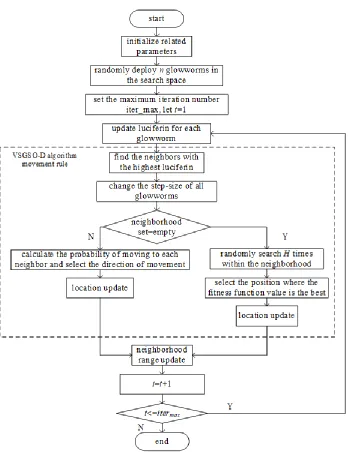
3.3VSGSO-D Algorithm Description

The main steps of VSGSO-D algorithm include initialization, luciferin update, step-size update, neighbor selection, movement, location update, and neighborhood range update (Fig. 1).

 iter_max t

()

round

H

( 1)

best

x t

J

i i

4. EXPERIMENTAL RESULTS AND ANALYSIS

4.1Experiment Platform

The experimental integrated development environment is MATLAB R2017a, the PC processor is Intel(R) Core (TM) i7-6700HQ, clocked at 2.60GHz, RAM is 8.00GB, and the operating system is 64-bit Windows 10.

4.2Experimental Preparation

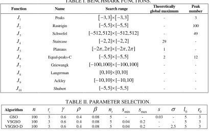
In this paper, ten benchmark functions of J₁ ~J₁₀ [7] are used to carry out algorithm optimization comparison experiments. Table.Ⅰlists relevant information of the ten benchmark functions. Table.II lists relevant parameter settings of algorithms. Ten benchmark functions are as follows:

2 2 2 2 2 2

1 2 1 2 1 2

[ ( 1) ] ( ) [( 1) )]

2 1 3 5

1 1 2 1 1 2

1

( , ) 3(1 ) 10( ) ( ) )

5 3

x x x x x x x

J x x  x e    x x e   e  

2 2

1

( ) (10 10 cos(2 ))

m

i i

i

J X x x







3

1

( ) 418.9829 sin( | |)

m

i i i

J X m x x



  



4( ,1 2) 25 1 2

J x x     _{   }x  x

5( ,1 2) (cos( ) cos( ))1 2

J x x sign x  x

2 2

6( ,1 2) cos ( ) sin ( )1 2

J x x  x  x

2

7

1 1

( ) 1 cos( )

4000 m m i i i i x x J X i    





1 1 1

1

( ) exp[ ( ) ]cos[ ( ) ]

p m m

i j ij j ij

i j j

J X c x a  x a



  









8

3 5 2 1 7

( : 5, 2, [1 2 5 2 3] , )

5 2 1 4 9

T T

J p m C A  _

 

2 9

1 1

1 1

( ) 20 exp 20 exp( 0.2 ) exp( 2 )

m m

i i

i i

J X x x

m  m  

   





5 5

10 1 2 1 2

1 1

( , ) cos(( 1) 1) cos(( 1) 1)

i i

J x x i i x i i x

 

TABLE I. BENCHMARK FUNCTIONS.

Function Name Search range Theoretically

global maximum

Peak number

1

J Peaks 3,3  3,3 - 3

2

J Rastrigin [ 5,5] [ 5,5]   - 100

3

J Schwefel [ 512,512] [ 512,512]   - 49

4

J Staircase [ 2, 2] [ 2, 2]   29 -

5

J Plateaus [ 2 , 2 ] [ 2 , 2 ]       1 -

6

J Equal-peaks-C [ 5,5] [ 5,5]   2 12

7

J Griewangk [ 100,100] [ 100,100]   - -

8

J Langerman [0,10] [0,10] - -

9

J Ackley [ 10,10] [ 10,10]   - -

10

J Shubert [ 5,5] [ 5,5]   - -

TABLE II. PARAMETER SELECTION.

Algorithm

GSO 100 3 0.6 0.4 0.08 5 - - 0.03 - 5 3

VSGSO 100 3 0.6 0.4 0.08 5 0.04 0.2 - - 5 3

VSGSO-D 100 3 0.6 0.4 0.08 5 0.04 0.2 - 2.5 5 3

Figure 1. VSGSO-D Algorithm Flow Chart.

4.3Experimental Results

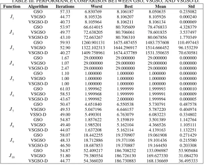
Thirty independent experiments are performed on the ten benchmark functions ~ , and three algorithms were compared, including the basic GSO and the VSGSO algorithm and VSGSO-D algorithm proposed in this paper. All test functions select the maximum value in their search space (Table. 1). Average iteration number,

the worst value, the best value, average value and standard deviation of optimization results are used as evaluation indexes of the algorithm optimization performance (Table. 3).

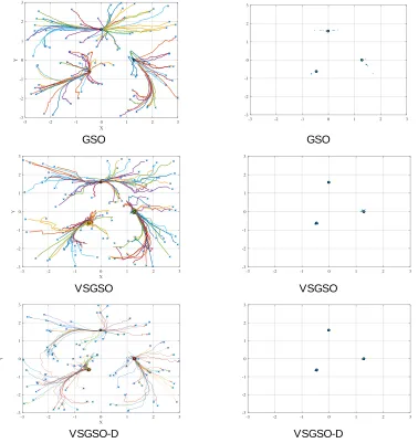
Trajectory and final location map of optimized J₁ of the basic GSO algorithm, the VSGSO algorithm and the VSGSO-D algorithm proposed in this paper are shown in Fig. 2. The relationship between the number of iterations and the function optimization value is shown in Fig. 3.

GSO GSO

VSGSO VSGSO

VSGSO-D VSGSO-D

Figure 3. The relationship between the number of iterations and the function optimization value. TABLE III. PERFORMANCE COMPARISON BETWEEN GSO, VSGSO, AND VSGSO-D.

Function Algorithm Iterations Worst Best Mean Std

1 J

GSO 57.33 6.830769 8.106187 8.050635 0.235082

VSGSO 44.77 8.105326 8.106207 8.105926 0.000240

VSGSO-D 40.73 8.105964 8.106211 8.106134 0.000069

2 J

GSO 53.97 66.614015 80.705609 78.476833 4.328379

VSGSO 49.77 72.638205 80.706061 78.601835 3.537497

VSGSO-D 43.10 72.663267 80.706310 80.067856 1.770349

3 J

GSO 59.93 1260.901131 1675.487455 1483.757608 110.497443

VSGSO 52.90 1322.102313 1644.296917 1514.666452 96.153239

VSGSO-D 40.27 1409.758961 1674.437789 1531.350635 70.630581

4 J

GSO 1.67 29.000000 29.000000 29.000000 0.000000

VSGSO 1.07 29.000000 29.000000 29.000000 0.000000

VSGSO-D 2.47 29.000000 29.000000 29.000000 0.000000

5 J

GSO 1.10 1.000000 1.000000 1.000000 0.000000

VSGSO 1.00 1.000000 1.000000 1.000000 0.000000

VSGSO-D 1.00 1.000000 1.000000 1.000000 0.000000

6 J

GSO 61.03 1.999962 1.999999 1.999993 0.000010

VSGSO 58.53 1.999968 1.999999 1.999991 0.000009

VSGSO-D 43.67 1.999982 2.000000 1.999994 0.000005

7 J

GSO 50.47 4.651840 6.550538 5.730791 0.487578

VSGSO 49.53 5.047196 6.646157 5.787220 0.404974

VSSO-D 49.00 5.490301 6.763079 6.083223 0.334802

8 J

GSO 54.87 1.857622 5.159819 3.501389 1.142764

VSGSO 49.40 1.985201 5.162104 4.366526 1.105111

VSGSO-D 44.07 1.637208 5.162114 4.139163 1.132251

9 J

GSO 58.07 18.442255 19.370907 19.061908 0.271429

VSGSO 48.33 18.712886 19.371106 19.101436 0.215580

VSGSO-D 46.50 18.687853 19.370887 19.164450 0.203308

10 J

GSO 54.87 52.409217 186.708232 133.096987 53.905684

VSGSO 51.80 79.380554 186.726130 169.627330 31.084270

4.4 Analysis of Results

VSGSO and VSGSO-D proposed in this paper are better than GSO in terms of the average number of iterations, precision, and stability of the results (Table. 3). In the optimization of discrete functions, the performance of the three algorithms are all good, and the VSGSO algorithm is the best in the iteration number. In the optimization of continuous multimodal functions, the performance of the VSGSO-D algorithm is the best. J₃ has high complexity in its search space. Comparing the results in the experiment (Table. 3), the advantage of the VSGSO-D algorithm is more obvious, which shows that it is also suitable to optimize high-dimensional complex multimodal functions.

1

J has three local maxima at positions (0, 1.58), (-0.46, -0.63), and (1.28, 0). From the glowworms’ trajectory and the final position map (Fig. 2), it can be seen that the VSGSO-D algorithm has the best local optimization precision. The GSO algorithm can capture three local peaks, but there are a large number of outliers.

Both the VSGSO algorithm and the VSGSO-D algorithm converge faster than the GSO algorithm, and the two algorithms proposed in this paper have shown apparent advantages in the early iteration (Fig. 3). It can be seen that the VSGSO-D algorithm has better convergence speed and optimization ability, and the curve is smoother, indicating that the current glowworm’s step-size and location have higher search efficiency for the target space.

5. CONCLUSIONS

ACKNOWLEDGMENTS

This work was supported in part by the National Key R&D Program of China under Grant 2016YFB1200602-26, in part by the National Key R&D Program of China under Grant 2016YFB1200601-B24.

REFERENCES

1. Fister, I., M. Perc, and S.M. Kamal. 2015. “A review of chaos-based firefly algorithms: Perspectives and research challenges,” Appl. Math. Comput., 252 (2015): 155-165.

2. Kaipa, K.N. and D. Ghose. 2017. Glowworm swarm optimization: Algorithm development. Glowworm Swarm Optim. Theory, Algorithms, Appl., 2017: 21-56.

3. Kaipa, K.N. and D. Ghose. 2017. Theoretical foundations,” Glowworm Swarm Optim. Theory,

Algorithms, Appl., 2017: 57-90.

4. Aljarah, I. and S.A. Ludwig. 2013. “A MapReduce based glowworm swarm optimization approach for multimodal functions,” 2013 IEEE Symp. Swarm Intell., 2013: 22-31.

5. Oramus, P. 2010. Improvements to glowworm swarm optimization algorithm. Comput. Sci., 11 (2010): 7-20.

6. Singh, A. and K. Deep. 2015. “New variants of glowworm swarm optimization based on step size,” Int. J. Syst. Assur. Eng. Manag., 6 (2015): 286-296.