An Improved Watershed Segmentation Method for Electron Microscopy Images

2018 International Conference on Computer Science and Software Engineering (CSSE 2018) ISBN: 978-1-60595-555-1

An Improved Watershed Segmentation

Method for Electron Microscopy Images

Qi Liu, Kaiyue Li, Guangtai Ding, Dongli Hu and Huiran Zhang

ABSTRACT

The analysis of nerve tissues is very helpful to the study of the nervous system. With the development and application of high-throughput technology, it becomes more important to realize the automated batch segmentation of nerve tissues in the electron microscopy(EM) image. Aiming at this, we propose an improved watershed segmentation method based on multiple deep-CNN models. Firstly, we use the classical watershed segmentation algorithm to obtain some candidate edge pixels in an original EM image. Secondly, the local regions of these candidate pixels are respectively extracted as the samples to be predicted. Thirdly, all candidate edge pixels are judged by a trained pixel classifier, of which the architecture is a deep convolutional neural network. Then, an initial segmentation result is generated based on the judgements. Finally, a complete segmentation image can be obtained after the morphological processing. The training and testing of model are finished on the ISBI dataset. The application of model is realized by merging the prediction results of three models with different scales. Experiments show that our method can spend less cost to have an approximate segmentation result, compared with other methods. Besides, our method can also show a better performance in the details.

INTRODUCTION

In nervous system, the information of individual neurons and their shapes are of value to the research of brain structured. The usual practice is to process and analyze the neuron images taken by serial-section Transmitted Electron Microscopy (ssTEM)[1]. After preparation of material researchers, the electron microscopy (EM) __________________________

image of neural tissue could be obtained. Due to the special preparation process and the different imaging principle, the classical image processing approach is very difficult to play a role in these images. With the development and application of high-throughput technology, the number of related images begins to increase rapidly. The need for reliable automated processing method is more urgent. Thus, the automatic segmentation has always been a research hotspot in the EM image of neural tissue.

The classic image segmentation algorithms usually have two application strategies: one is the edge extraction method based on some edge detection operators, like Sobel [2] and Laplacian [3]; the other is the region segmentation method based on some similarity measurements, like watershed [4]. Threshold segmentation method is an application example of the former strategy [5,6]. Region growth method is an application example of the latter strategy [7,8]. Although these methods can achieve some certain effects in electron microscope images, they are not real automatic segmentation methods strictly. The choice of most parameters in these methods always depends on a lot of prior knowledge.

In recent years, deep neural network has demonstrated their effectiveness in many visual tasks [9-11]. In the segmentation of medical EM image, there are two popular network architectures based on local and global. The Convolutional Neural Network(CNN) [1] architecture completes the pixel classification by processing the local information of an image. The Fully Convolutional Network(FCN) [12] architecture is based on the global information to directly generate the final processing result. The CNN model has a higher cost and redundancy during the processing of segmentation task, because all pixels in an image are treated equally. The FCN model requires a large amount of data for parameter training. Many training samples can be produced by using elastic deformation [13]. The convolution operations in the FCN is finished based on the local information. The truth is, elastic deformation cannot drastically change the local information of an image. Therefore, it is too difficult to prove that increased samples are really helpful to model training, rather than just increase the number of samples [14].

classification. Experiments show that our method performs better than other methods in computational cost and segmentation effect.

METHOD

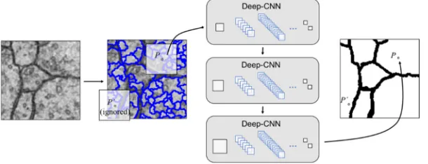
The watershed algorithm can complete the initial segmentation in the electron microscope image. The purpose is to divide the image into many small non-overlap regions as much as possible. These inter-region edges already contain all edges of nervous tissues in the EM image because of over-segmentation. Therefore, we trained a deep-CNN model to determine which edge pixels need to be removed. In other words, the model is designed to obtain a whole nervous tissue by achieving region merging. Our method flow is shown in Figure 1. The edge pixels in the initial segmentation are called as candidate edge pixels. The deep model just classifies these candidate edge pixels, that is, to find out the real edge pixels among them. Since it is a pixel level processing task, we would like to use the morphological processing for optimizing the final segmentation result.

Watershed Segmentation

The watershed segmentation algorithm is used to complete the preprocessing of original images. Firstly, we calculate pixel gradients of an image by the edge detection operator[2,3]. Secondly, we select some pixels with smaller gradients in the image as the seed points of region growing. Thirdly, we simulate to fill the water from each seed points, until the contour of corresponding local region is found. Finally, the watershed segmentation result of whole image can be obtained.

Deep-CNN Architecture

The deep CNN has been shown to be valuable in some tasks such as image classification[11] and image segmentation[1]. These network architectures are typically similar, consisting of a large number of convolutional layers, pooling layers and fully connected layers. The model based on the FCN architecture also contains a series of deconvolutional layers[14]. The core of these architectures is to extract the deep image features through the convolution operations. Thus, the purpose of model training is to use the loss optimization to fit all weight parameters applied in the convolution operations[15].

The deep network presented in this paper aims to determine the pixel category and realize the region merging. We only judge all candidate edge pixels obtained by the watershed segmentation algorithm. For the obvious background pixels, we don't need to spend much computing cost in the deep model again. Therefore, the architecture design of deep network can be simpler and more direct. The biggest architectural difference between our deep model and other deep neural network[1] is the ratio between the numbers of convolutional layers and pooling layers[16-18]. Since the data object of model is the local regions of an image, the size of input image sample is small. We would like to use less pooling layers. This ensures that the last convolutional layer can have an enough receptive field to perceive the information.

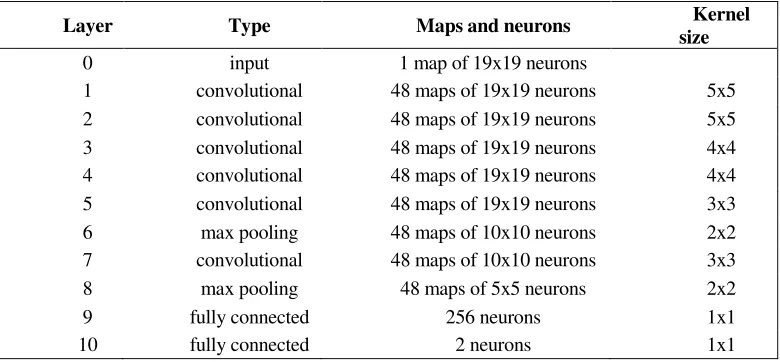
The architecture of our model is shown in Table I. The model consists of 11 layers, including an input layer, six convolutional layers, two pooling layers, and two fully connected layers. The model shown in Table I is designed for the input image sample of shape 19x19. The shape of input image sample can be modified under the premise that the model architecture is unchanged. Certainly, the neuron shape of middle layer will be changed at the same time. No matter how we change the input image sample, the output of model is always a 2d vector. We use this vector to determine whether the current pixel is a real edge pixel.

TABLE I. MODEL ARCHITECTURE.

Layer Type Maps and neurons Kernel

size

0 input 1 map of 19x19 neurons

Training

For training the pixel classifier, we use the electron microscopy images in the ISBI Challenge dataset[19,20]. The watershed segmentation algorithm is applied to the whole image. The deep-CNN model is applied to the local region of image. Unlike other methods, we would not predict the categories of all pixels in the image. Only edge pixels obtained by the watershed segmentation are processed in the deep model.

The ISBI dataset provides many images with a 512x512 resolution. We segment out all edge pixels and their neighborhood regions from a preprocessed image. These local regions are used as the image samples for subsequent training. If the center pixel of a region sample is indeed an edge pixel, this sample is a positive sample; otherwise, it's a negative sample. In this way, an image with a 512x512 resolution can produce about tens of thousands of samples. The obvious background pixels are not in the deep model's consideration at all. Due to the sufficient sample size, we do not need to use other means to increase sample number.

In order to improve the accuracy and robustness of model prediction, we slightly adjusted the structure of deep model during training. We respectively added the noise layer[21] on the front of the 2th and 3th layers of the model. The noise layer was used to add the Gaussian noise(with the mean of 0 and the variance of 0.05) into the sample data. In addition, we respectively added the batch normalization layer[22] on the front of the 4th, 5th, 7th and 9th layers. These added layers are just used during the training phase. They can accelerate convergence and avoid overfitting.

Postprocessing

Because the pixel classification is applied based on the watershed segmentation result, some edges may appear the phenomena such as branching and non-closing. We use morphological processing[23] to accomplish the work of pruning and clogging. After a successful implementation of subsequent processing of one image, these processing parameters can be extended to all images of the same kind. Finally, a series of complete segmentation results of neural tissues can be obtained.

EXPERIMENTS

To ensure that most of the real edge pixels could be marked as candidate edge pixels, we used morphological dilation on the watershed segmentation result. This could make more pixels to participate in the next phase of classification prediction. We trained three models, with same architecture and different shapes of input window. During the training, we used the RELU activation function, the Binary Cross-Entropy loss function and the ADAM optimizer[24]. The training results of deep model are shown in Table II. Data suggests that our model can achieve a good result on pixel-level accuracy.

All experiments were performed on a computer with a Core(TM) i7-8700 3.20GHz processor, 16GB of RAM, and one GTX 1060 graphics card(6GB). The software part of the method used the GPU acceleration [25]. Based on the watershed segmentation, the computing cost of our method could be saved over 70%, compared with other methods. The comparisons of hardware usage and model speed are shown in Table III. It visually shows the advantages of our method in the usage time of training and testing. Besides, the cost of hardware consumption is also lower in the realization process of our method.

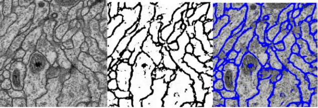
The segmentation of test images was accomplished through three deep models. We referred to the combination of three models as the Average Deep Model(ADM). The ADM determined the real edge pixels based on the votes of three models. The final segmentation result of test image completed by ADM is shown in Figure 2. Under the premise of saving more than half of computing resources, our method can achieve the same segmentation effect as other methods [1,14]. In the details, our method can produce less noise and get better performance.

TABLE II. TRAINING RESULTS.

Accuracy

pixel-level

Model 1

Input Size 15

Model 2

Input Size 19

Model 3

Input Size 23

training 96.16% 96.57% 97.39%

testing 94.42% 95.23% 96.02%

TABLE III. COMPUTING COST.

Approach Hardware usage Training time /

epoch

Testing time / image

Our model four GTX 580 graphics

cards 12min-18min 18sec-32sec

Figure 2. The slice 16 of the test stack and its segmentation result.

CONCLUSIONS

Our deep classification model is used to optimize the pre-segmentation results of the watershed algorithm, rather than to complete an end-to-end segmentation task. Compared with other methods, our approach can use much fewer sample images, so as to improve the efficiency of training and prediction. The other advantage of our approach is to use the processing results of traditional algorithms as the prior knowledge used in the design and training of deep model. In addition to solving the segmentation task of EM images of nerve tissues, it also provides a certain reference value and significance for addressing other EM images.

ACKNOWLEDGMENT

This work is supported by the National Key Research and Development Program of China (No.2016YB0700502).

REFERENCES

1. Dan C C, Giusti A, Gambardella L M, et al. Deep Neural Networks Segment Neuronal Membranes in Electron Microscopy Images. Advances in Neural Information Processing Systems, 2012, 25:2852-2860.

2. Gao W, Zhang X, Yang L, et al. An improved Sobel edge detection. IEEE International Conference on Computer Science and Information Technology. IEEE, 2010:67-71.

3. Dokkum P G V. Cosmic-Ray Rejection by Laplacian Edge Detection. Publications of the Astronomical Society of the Pacific, 2001, 113(789):1420-1427.

4. Nguyen H T, Worring M, Boomgaard R V D. Watersnakes: Energy-Driven Watershed Segmentation. Pattern Analysis & Machine Intelligence IEEE Transactions on, 2003, 25(3):330-342.

5. Belhomme P, Houivet D, Lecluse W, et al. Image analysis of multiphased ceramics. Journal of the European Ceramic Society, 2001, 21(10–11):2149-2151.

7. Banerjee S, Datta S, Paul B, et al. Segmentation of three phase micrograph:an automated approach. Cube International Information Technology Conference. 2012:1-4.

8. Park J K, Lee S H. Observation and Segmentation of Gray Images of Surface Cells in Open Cellular Ceramic Foams. Journal of the Ceramic Society of Japan, 2001, 109(1271):580-586. 9. Cireşan D C, Meier U, Gambardella L M, et al. Deep, big, simple neural nets for handwritten

digit recognition. Neural Computation, 2010, 22(12):3207-3220.

10. Dan C C, Meier U, Gambardella L M, et al. Convolutional Neural Network Committees for Handwritten Character Classification. International Conference on Document Analysis and Recognition. IEEE Computer Society, 2011:1135-1139.

11. Schmidhuber J. Multi-column deep neural networks for image classification. Computer Vision and Pattern Recognition. IEEE, 2012:3642-3649.

12. Long J, Shelhamer E, Darrell T. Fully convolutional networks for semantic segmentation. IEEE Conference on Computer Vision and Pattern Recognition. IEEE Computer Society, 2015:3431-3440.

13. Schaefer S, Mcphail T, Warren J. Image deformation using moving least squares. ACM SIGGRAPH. ACM, 2006:533-540.

14. Ronneberger O, Fischer P, Brox T. U-Net: Convolutional Networks for Biomedical Image Segmentation. International Conference on Medical Image Computing and Computer-Assisted Intervention. Springer, Cham, 2015:234-241.

15. Lecun Y, Bottou L, Bengio Y, et al. Gradient-based learning applied to document recognition. Proceedings of the IEEE, 1998, 86(11):2278-2324.

16. Riesenhuber M, Poggio T. Hierarchical models of object recognition in cortex. Nature Neuroscience, 1999, 2(11):1019.

17. Scherer D, Müller A, Behnke S. Evaluation of Pooling Operations in Convolutional Architectures for Object Recognition. International Conference on Artificial Neural Networks. Springer-Verlag, 2010:92-101.

18. Serre T, Wolf L, Poggio T. Object Recognition with Features Inspired by Visual Cortex. IEEE Computer Society Conference on Computer Vision & Pattern Recognition. IEEE Computer Society, 2005:994-1000.

19. Argandacarreras I, Turaga S C, Berger D R, et al. Crowdsourcing the creation of image segmentation algorithms for connectomics. Frontiers in Neuroanatomy, 2015, 9:142.

20. Cardona A, Saalfeld S, Preibisch S, et al. An Integrated Micro- and Macroarchitectural Analysis of the Drosophila Brain by Computer-Assisted Serial Section Electron Microscopy. 2010, 8(10): e1000502.

21. Srivastava N, Hinton G, Krizhevsky A, et al. Dropout: a simple way to prevent neural networks from overfitting. Journal of Machine Learning Research, 2014, 15(1):1929-1958.

22. Ioffe S, Szegedy C. Batch normalization: accelerating deep network training by reducing internal covariate shift. International Conference on International Conference on Machine Learning. JMLR.org, 2015:448-456.

23. Angulo J, Velasco-Forero S, Bloch I, et al. Mathematical Morphology and Its Applications to Image and Signal Processing. Computational Imaging & Vision, 2011, 6671(4):384.

24. Kingma D, Ba J. Adam: A Method for Stochastic Optimization. Computer Science, 2014. 25. An D C, Meier U, Masci J, et al. Flexible, high performance convolutional neural networks for