INERT STATE SOLUTION OF IGNITION AND FLAME STRUCTURE
BEHIND SHOCK PROPAGATING INTO A REACTIVE GAS
Mushtaq A. Khan1, Adem H. Ibrahim2
1Department of Mathematics, Norfolk State University, Norfolk, Virginia, USA 2Engineering Department, Norfolk State University, Norfolk, Virginia, USA
ABSTRACT
The non-dimensional Continuity, Momentum, Energy, Mass-Fraction equations and Equation of
State governing the two-dimensional, unsteady motion of a compressible, reacting gas in the
boundary layer to the leading order in a Reynolds number are derived. The resulting coupled
momentum and energy equations are numerically solved for both adiabatic and isothermal
boundary conditions with different values of the independent parameters like Mach number,
surface temperature and Prandtl number. The effect of these parameters on temperature and
velocity profile are presented. For comparison purposes, the inert-state problem for the linear
temperature viscosity law is also solved for different values of independent parameters.
KEY WORDS: Adiabatic boundary, isothermal boundary, boundary layer, shock wave,
Rankine-Hugoniot condition, Mach number, Prandtl number, Temperature-Viscosity laws, COLSYS
INTRODUCTION
In the flow behind the shock front [1, 2, 3, 4, 5, 6, 7, 8, 9], there exists an inert heating stage prior to the events that lead to ignition. On this inert state, the flow is self-similar. The inert-stage momentum, energy and mass-fraction equations are derived. The solution to these equations is determined numerically for both the adiabatic boundary conditions, with no transfer of heat across the wall, and the isothermal boundary conditions, with the wall temperature held constant. For comparison purposes, the inert-state problems are solved for different values of independent variables, using both linear temperature-viscosity law and Sutherland’s law. The results are
International Research Journal of Natural and Applied Sciences
ISSN: (2349-4077) Impact Factor- 5.46, Volume 4, Issue 10, October 2017 Website- www.aarf.asia, Email : [email protected] , [email protected]
Governing Equations
The non-dimensional equations to the leading order in a Reynolds number expansion that govern the two-dimensional, unsteady motion of a compressible, reacting gas in the boundary layer are given by:
Continuity Equation
( ) ( )
+ ˆ ˆ =0+ x y
t ρu ρv
ρ , (1.1)
Momentum Equation
[
t x y]
px( )
uy yM u
v uu
u ˆ 2 ˆ ˆ
1
ˆ µ
γ
ρ + + + = (1.2)
Energy Equation
[
Tt uTx vTy]
(
Pt+uPx)
− − + +
γ γ
ρ ˆ ˆ 1 =
( )
µ +(
γ −)
µ( )
2 +βΩˆ 2 ˆ
ˆ 1
1
y y
y r
u M T
P , (1.3)
Mass-Fraction Equations
[
+ +]
=( )
−Ωy y e y
x
t Y
PL Y
v uY
Y ˆ ˆ ˆ
1
ˆ µ
ρ , (1.4)
Equation of State
T
P=ρ . (1.5)
T is the temperature, ρ is the density, P is the pressure and Y is the mass fraction of the deficient
reactant in the combustible gas. The reaction is modeled as a simple, single-step, irreversible reaction.
The x-axis is taken in the direction of the flow and tangent to the wall; the y-axis is
normal to the wall. The velocity component u is tangent to the wall, and vˆ is the properly scaled component normal to the wall. In the derivation of the above system of equation, the scaled boundary-layer variables
y R y
e ˆ 1
= , and v
R v
e ˆ 1
= (1.6)
have been introduced in order to study the effects of chemistry in the boundary layer. Balancing
The dimensionless variables are obtained by selecting ' 0 T , '
0 Y , '
0 ' 0 u L , ' 0 ' 0RT
ρ , and ' 0
L to be
the units of temperature, mass fraction, time, pressure and length respectively. For convenience,
' 0 T , '
0
ρ and ' 0
u are chosen to be the free stream values behind the shock and are also denoted by
'
∞
T , ρ∞' and u∞' . Thus '
' ∞ ∞ = a u
M is the Mach number of the gas (piston) pushing the shock front,
and '
∞
a is the speed of sound in the gas behind the shock front. The remaining non-dimensional
quantities are the Prandtl number
' 0 ' ' 0 k c
Pr = µ p , (1.7)
the ratio of specific heat of a gas at constant pressure to that at constant γ , and the Reynolds
number Re
' 0 ' 0 ' 0 ' 0 ρ µ u L
Re = , >> 1 (1.8)
The heat release parameter β and the reaction term Ω are
' 0 ' ' 0 ' T c Y Q p =
β and Ω=DρYe−ET (1.9)
Where ' 0T0' R E
E= is the activation energy and ' ' 0 ' ' 0 ' 0 D t D u L
D= = is the Damkohler number,
with '
D being the pre-exponential factor. Presently, the parameterD is arbitrary and making a
choice implies a choice of the length scale. If D isO(1), then Ω→0 in the limitE→∞, and the
reaction term is zero at all algebraic orders. This suggests that D be chosen as
∗
= T
E
e D
D 0εδ (1.10)
where D0, δ , and
∗
T are determined later in the analysis. The length scale of the problem is now
given as ∗ = T E e D D u
L ' 0εδ
' 0 '
It is noted that the expression for D does not determine the characteristic length until the
temperature T∗ has been specified. If T∗ is > 1, the characteristic length is much shorter than the outer explosion distance (i.e., the distance between the shock and an insulated piston at thermal runaway; see Jackson et al. [12]). In addition, if the distance between the shock and the piston face is much greater than the thickness of the boundary layer, the chemical effects are initially confined to the boundary layer with the outer flow being essentially inert. This allows the study of the “steady state” which develops in the boundary layer directly behind the shock. For a general discussion of activation energy asymptotic, see Buckmaster[3].
Variable Transformation
The mean flow equations (1.1) – (1.5) are first transformed to the incompressible equations by means of the Howarth-Dorodnitsyn transformation through the change of variables
(
)
' 0'
, ,y tdy x
y
∫
= ρ
ξ , x =x and t =t (2.1)
Then another change of variables is introduced
x t u
u
s s
−
= ξ
η , X =ust −x , and t =t (2.2)
Where η is the similarity variable. The transformation in X means that the equations are relative
to a new coordinates system in which the shock front is stationary and the fluid moves towards the
shock front at a constant speed us. This speed us is found in terms of the Mach number M of the
piston speed to be
(
)
(
)
M M M
us
4
16 1
3− + − 2 2 +
= γ γ (2.3)
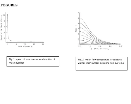
This relationship is derived from Rankine-Hugoniot condition. Figure 1 shows the shock speed us
versus the Mach numberM . Note that us →∞ asM →0, and for largeM, the shock speed
1
→
s
u . In reality, us measures the speed of traveling discontinuity that is initiated by the
instantaneous movement of the piston. This discontinuity is not formally a shock wave unless the speed of the discontinuity is greater than the speed of sound in the undisturbed gas. This condition for a formal shock wave to exist is equivalent toM >1. Also, it is known that a small disturbance
in the limit of zero Mach number travels at the speed of sound; the asymptotic relation
as M →0 is consistent with this fact since in dimensional units this asymptotic relation gives ' ' ' ' ~ ∞ ∞ ∞ u a u us
. The resulting continuity equation is solved for
( )
ρvˆη and both sides integrated withrespect to η to getρvˆ.
η η
η ξ
ξ
ρ =− − − η
∫
′ η′ ′+ η∫
u d ′u X d u X u u v X s s x t 0 02 1 1 (2.4)
The resulting momentum, energy, and mass-fraction equations are
Momentum Equation
(
)
(
η)
ηη
η η
η
η η η µρ
η u X u d u u ud X u u X u u u u
u + s − X − s +
∫
′+∫
X ′= s0 0 2 2 (2.5) Energy Equation
(
−)
− +∫
′+∫
′=+ η η η η η η
η ud T u d
X T T X u T u u
T s X
X s t 0 2 2
(
)
+(
−)
( )
( )
+ Ωρ β µρ
γ
µρ η η 2 η 2
1 1 u X u M T X u P s s r (2.6) and Mass-Fraction Equation
(
−)
− +∫
′+∫
′=+ η η η η η η
η ud Y u d
X Y Y X u Y u u
Y s X
X s t
0
2
2
(
µρ η)
η − ρΩ1 1 Y X u L P s e r (2.7)
Which along with the equation of the state 1
=
T
ρ (2.8)
provide a closed system for the unknownu, ρ, T and Y.
In these equations, the quantitiesξt, ξx and ξxu are
η ρ ρ ρ ρ ρ ρ η ρ ρ ξ
ξ η η η ′
+ + ′ −
=
∫
′ du X u X u X u t s X s s s t t 2 1 0 (2.9) η ρ ρ ξ ρ ρ ρ ρ η
ξ η η ′
η ξ ρ ρ ξ ρ ρ ρ ρ η
ξ η η η η ′
+ + − ′
=
∫
′ u ′ u ′ du X u X u u
u x x
X s s x 0 2 1 (2.11)
Inert State Equations
In the flow behind the shock front, there exists an inert heating stage prior to the events that lead to ignition. On this inert state, the flow is self-similar and it is assumed that the solution is independent of X and t. To get the momentum and energy equations for the inert state, we let
(
η,X,t)
uI( )
η ,u = T
(
η,X,t)
=TI( )
η and Y(
η,X,t)
=YI( )
η in equations (2.5), (2.6) and (2.7). Thesubscript I denotes the inert-state dependent variables. The stream-function f
( )
η is introduced bylettinguI
( )
η → f′( )
η . The appropriate change of variables is used to transform the momentumequation to the form of IM et al. [10].
The momentum and energy equations for the inert state are
(
η)
ηη
η I η sη s µρ I
I u d u u u
u 2 0 = − ′
∫
(3.1) and( )
[
]
(
)
2[
2]
0 1 2 1 η η η η η µρ γ µρ η η
η I s I
r s I s
I T u M u
P u T u d
u = + −
− ′
∫
(3.2)Subject to the boundary conditions
( )
0 =0 Iu ,uI
( )
∞ =1, and TI( )
∞ =1 (3.3)( )
sI T
T 0 = for isothermal wall, and
( )
0 =0η d dTI
, for adiabatic wall (3.4)
In the adiabatic case, the wall at η =0 is insulated so that there is no transfer of heat across that
surface; whereas, in the isothermal case, the wall at η =0 is held constant at some temperatureTs
. The mass-fraction equation is trivially solved to the conditions YI
( )
∞ =1 and YIη( )
0 =0 to get( )
η =1 IY (3.5)
Letting uI
( )
η = f′( )
η and denoting µρ byµ, the momentum equation becomes(
f −usη)
f ′′=2us( )
µf ′′η, (3.6)Subject to
( )
0 =0f , f′
( )
0 =0, and f′( )
∞ =1 (3.7)( )
[
]
[ ]
(
)
2[ ]
21 2
1
f M u
T P u T u
f I s
r s I
s = + − ′′
− η µ γ µ
η η η η (3.8)
subject to the same boundary conditions as above.
The momentum equation (3.6) is not independent of the energy equation since the term µ
is a function of temperature. In case of IM et al. [10], the linear temperature-viscosity law is used (µ =1 ); the momentum equation decouples from the energy equation; and the velocity field is
determined independently.
For comparison, it is convenient to transform the equations to the form of IM et al [10] using the change of variables
F u u
f − sη =− 2 s , and η= 2usη (3.9)
The momentum equation is now
− = F
F
µF , (3.10)
Subject to
0 ) 0 ( =
F , F(0)=us and F(∞)=us −1 (3.11)
where () is for η
d d
.
Similarly, the energy equation for the inert state in terms of η is
[
]
(
)
2[
2]
21 1
F f T M TT
P
FT I I
r
I = + − ′′
− η µ η η γ µ (3.12)
subject to
( )
∞ =1 IT ,
( )
0 =0η d dTI
for adiabatic wall,TI
( )
0 =Ts for isothermal wall (3.13)We note here that the governing equations are identical to the governing equations of IM et al,
[10], except that they have F(0)=0 and F(∞)=1 as a boundary conditions andµ =1. For
comparison, these governing equations are solved using the boundary conditions of Im et al. [10]
andµ =1. This is referred to as the linear temperature-viscosity law with us =0 case. Also, solved
are these governing equations using the boundary conditions of IM et al [10] and µ computed
through Sutherland’s temperature-viscosity law. This is referred to as the Sutherland’s law with
referred to as the linear temperature-viscosity law with us ≠0 case, and the solution for µ
computed through the Sutherland’s temperature-viscosity law is referred to as the Sutherland’s
law with us ≠0 case. The results of all the four cases with different set of the physical parameters
are discussed below.
Results and Analysis
The coupled momentum and energy equations (3.10) and (3.12) are numerically solved using COLSYS for both adiabatic and isothermal boundary conditions with different values of the independent parameters like Mach number, surface temperature and Prandtl number. For comparison purposes, the inert-state problem for the linear temperature-viscosity law is also solved for different values of the independent parameters. In addition, the inert-state problem for both the Sutherland’s law and the linear temperature-viscosity law are solved for the boundary conditions in Im et al. [10]. Results for the adiabatic boundary conditions, where there is no transfer of heat
across the surface at η =0, are shown in Figure 2 through 7. Figure 2 shows the temperature
( )η −1
I
T versus η for various values of Mach number increasing from M=0.5 to M=5 and unit
Prandtl number. The speed of shock wave us is calculated from equation (2.3). Note that, as the
Mach number increases, there is a corresponding increase in the maximum inert temperature occurring at the boundary near η =0 due to viscosity heating. This quantity will be referred to as
the adiabatic surface temperatureTad. The thickness of this thermal layer is terms of the similarity
variable η remains relatively constant.
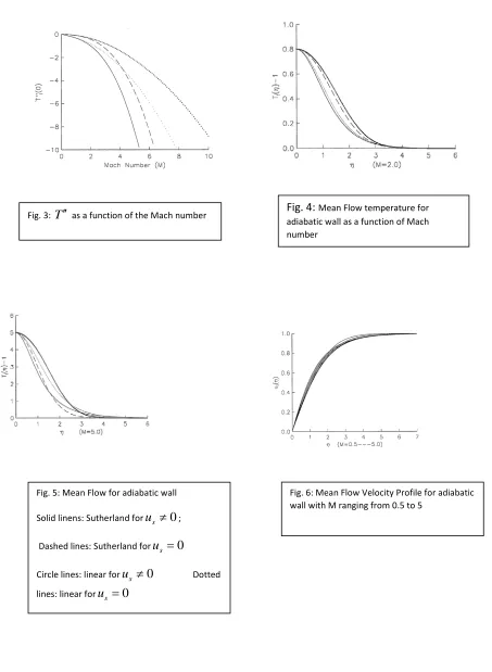
In Figure 3, TI
( )
0 versus Mach M shows the significant increase in the magnitude of the( )
0 IT for large Mach numbers. For comparison, the graph of TI
( )
0 versus Mach number is shownfor the four different problems mentioned. Solid and dash curves show the results of using the
Sutherland’s temperature-viscosity law. The shock speed us has been calculated from equation
(2.3) (solid curve) and has also been set to zero (dashed curve). The dotted and circle curves show
the results of using the linear temperature-viscosity law with us ≠0and with F(0)=0 and
1 ) (∞ =
F ; for brevity, this will hereafter be referred to as the us ≠0 case. The magnitude of the
4 and Figure 5 by plotting the inert-state temperature TI
( )
η −1 versus η for these four cases. TheMach number M=2.0 is used for Figure 4 and M=5.0 is used for Figure 5. The difference is more significant for a larger Mach number. Note that, although the adiabatic wall-temperature is the same for a constant Mach number, changing from linear temperature-viscosity law to the
Sutherland’s temperature-viscosity law and changing from us =0 to the shock speed us calculated
through the Rankine-Hugoniot relations localizes the viscous heating near the boundary. On this point alone, it is seen that the ignition results found here differ substantially from IM et al [10].
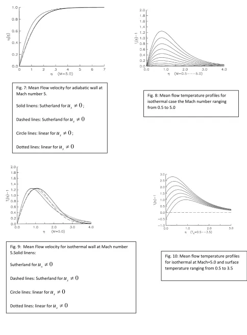
Figure 6 shows velocity uI
( )
η versus η for different values of the Mach number and unitPrandtl number. Figure 7 shows uI
( )
η versus η for Mach number M=5.0 for the above four cases.The solid and dashed curves are for the Sutherland’s law with us ≠0 andus =0, respectively. The
dotted and circle curves are for the linear temperature-viscosity law with us ≠0 andus =0,
respectively. The graph shows no difference between the velocity profiles for the us ≠0 and the
0
=
s
u case. This is quite interesting since it is the velocity profiles that govern the creation of
thermal energy through viscous heating. The major differences in the results for the us ≠0 and
the us =0 cases are due to the difference in the convective terms only. These differences show up
in the temperature profiles as seen in Figures 4 and 5. Along with the previous differences noted
in the second derivative of the temperature at the wall surface, it is found that us ≠0 and the Mach
number is relatively large, the temperature profile is broader than the us =0 case when each are
considered using the appropriate similarity variable. This should be noted that a direct comparison is not necessarily proper since, in the two cases, the similarity variables represent different quantities, however, the overlapping of the two velocity profiles in their respective variables merit the special mention given here.
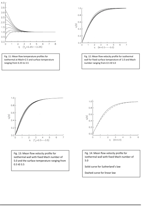
The system of equations (3.10) and (3.12) are also solved for the isothermal boundary
conditions where the surface temperature is kept at a constant temperatureTs. In the isothermal
wall case, there are two varying parameters, namely, the Mach number M and the surface
temperatureTs. The effects of both parameters are analyzed by keeping one of them constant and
varying the other. Also, for comparison purposes, the problem is solved for the linear
conditions, to the us =0 case. Figure 8 shows the temperature TI
( )
η −1 versus η for differentvalues of Mach numbers ranging from M=0.5 to M=5.0 with surface temperature Ts =1 and unit
Prandtl number. The speed,us of the shock front, is calculated from equation (2.3). The plot shows
that the maximum temperature lies in the interior of the boundary layer and the maximum value increases as the Mach number increases. It also shows that the effect of the Mach number on the
location of the maximum temperature is not very significant. Figure 9 is a plot of TI
( )
η −1 versusη , for fixed Mach number M=5.0, surface temperature Ts =1.0 and Prandtl number,Pr =1.0.
Solid and dashed curves show the results of using the Sutherland’s temperature-viscosity law. The
solid curve is for uscalculated from equation (2.3) and the dashed curve is for the us =0 case.
The dotted and circle curves show the results of using the linear temperature-viscosity law for the
0
≠
s
u case, respectively. The plot shows a shift in the position of the maximum temperature
location between theus ≠0, and us =0 cases. Figure 10 shows the temperature TI
( )
η −1 versusη for fixed the Mach number M=5.0 and with the surface temperature increasing from Ts =0.5
to Ts =3.5. The effect of the surface temperature Ts on temperature profiles is shown in Figure
11 for fixed Mach number, M=2.5. If the value of the surface temperature Ts is greater than the
adiabatic valueTad, then the temperature attains its maximum at the boundary, η =0. Figure 12
shows the velocity uI
( )
η versus η for different values of the Mach number. It is determined thatthe velocity profile does not vary much with the Mach number M. The effect of surface temperature on the velocity profiles is shown in Figure 11 for fixed Mach number M=5.0. In Figure 12, velocity profiles for the Sutherland’s and linear temperature-viscosity law are shown. The solid curve denotes the use of the Sutherland’s law and the dotted curve denotes the use of the linear law.
CONCLUSION
The coupled momentum and energy equations are numerically solved using COLSYS for both adiabatic and isothermal boundary conditions with different values of the independent parameters like Mach number, surface temperature and Prandtl number. It is noted that, for adiabatic wall, as the Mach number increases, there is a corresponding increase in the maximum inert temperature
is terms of the similarity variable η remains relatively constant. Also, the magnitude of the second
derivative of the inert-state temperature near the boundary for the Sutherland’s viscosity law is significantly larger than for the linear temperature-viscosity law, especially for large Mach numbers. This indicates a more localized viscous heating. It is very important to note that, although the adiabatic wall-temperature is the same for a constant Mach number, changing from linear
temperature-viscosity law to the Sutherland’s temperature-viscosity law and changing from us =0
to the shock speed us calculated through the Rankine-Hugoniot relations localizes the viscous
heating near the boundary. On this point alone, it is seen that the ignition results found here differ substantially from IM et al [10]. For isothermal wall, the plot shows that the maximum temperature lies in the interior of the boundary layer and the maximum value increases as the Mach number increases. It also shows that the effect of the Mach number on the location of the maximum temperature is not very significant. It is also determined that the velocity profile does not vary much with the Mach number M.
[image:11.612.70.518.326.684.2]FOGURES
Fig. 1: speed of shock wave as a function of
Fig. 3: T′′ as a function of the Mach number Fig. 4: adiabatic wall as a function of Mach Mean Flow temperature for number
Fig. 5: Mean Flow for adiabatic wall
Solid linens: Sutherland forus ≠0;
Dashed lines: Sutherland forus =0
Circle lines: linear forus ≠0 Dotted
lines: linear forus =0
[image:12.612.330.507.76.279.2][image:13.612.65.549.27.682.2]
Fig. 7: Mean Flow velocity for adiabatic wall at Mach number 5.
Solid linens: Sutherland forus ≠0;
Dashed lines: Sutherland forus ≠0
Circle lines: linear forus ≠0;
Dotted lines: linear forus ≠0
Fig. 8: Mean flow temperature profiles for isothermal case the Mach number ranging from 0.5 to 5.0
Fig. 9: Mean Flow velocity for isothermal wall at Mach number 5.Solid linens:
Sutherland forus ≠0
Dashed lines: Sutherland forus ≠0
Circle lines: linear forus ≠0
Dotted lines: linear forus ≠0
[image:14.612.87.545.31.700.2]
Fig. 11: Mean flow temperature profiles for
isothermal at Mach=2.5 and surface temperature ranging from 0.25 to 3.5
Fig. 12: Mean flow velocity profile for isothermal wall for fixed surface temperature of 1.0 and Mach number ranging from 0.5 t0 5.0
Fig. 13: Mean flow velocity profile for isothermal wall with fixed Mach number of 5.0 and the surface temperature ranging from 0.5 t0 3.5
Fig. 14: Mean flow velocity profile for isothermal wall with fixed Mach number of 5.0
Solid curve for Sutherland’s law
REFERENCES
1. R. P. Benedict (1993), Fundamentals of Gas Dynamics, John Wiley and Sons, 30-33. 2. J. N. Bradley (1962), Shock Waves in Chemistry and Physics, John Wiley and Sons.
3. J. D. Buckmaster (1985), The Mathematics of Combustion. SIAM.
4. S. I. Cheng and A.A. Kovitz. Ignition in the Laminar Wake of a Flat Plate. 6th Symp. (Intl.) Combustion, Reinhold, 1957, pp. 418.
5. S. I. Cheng and A.A. Kovitz. Mixing and Chemical Reaction in the Laminar Wake of a Flat Plate. Journal of Fluid Mechanics, 1958, Vol. 4, pp. 64.
6. J.F. Clarke and R. S. Cant (1984), Nonsteady Gasdynamics Effects in the Induction Domain Behind a Strong Shock Wave. Progress in Aeronautics and Astronautics.
7. D. A. Dooley (1956), Ignition in the Laminar Boundary Layer of a Heated Plate. Heat Transfer and Fluid Mechanics Ins., Stanford University Press, 321-342.
8. Silva da Figueira, Deshaies, L. F. and Champion, M. (1993), “Numerical Study of Ignition With in Hydrogen-Air Supersonic Boundary Layer”, AIAA Journal, Vol. 31, No. 5.
9. Grosch, C. E., and JacksonT. L. (1991), “Ignition and Structure of a laminar Diffusion Flame in a Compressible Mixing Layer with Finite Rate chemistry”, Phys. Fluids A, Vol. 3, No. 12, pp. 3087-3097.
10. Im,H. G. , Bechtold, J. K., and Law C. K., (1993), “Analysis of Thermal Ignition in Supersonic Flat-Plate Boundary layers”. Journal of Fluid Mechanics, Vol. 249, pp. 99-120.
11. Jackson,T. L., and Hussaini, M. Y, (1988), “An Asymptotic Analysis of Supersonic Reacting Mixing Layers”. Combustion Sci. Tech, Vol. 57, 1988, Nos. 4-6, pp. 129-140.