R E S E A R C H
Open Access
Exponential stability analysis of nonlinear
systems with bounded gain error
Xingkai Hu
1,2*and Linru Nie
1,2*Correspondence: [email protected] 1Faculty of Civil Engineering and
Mechanics, Kunming University of Science and Technology, Kunming, P.R. China
2Faculty of Science, Kunming
University of Science and Technology, Kunming, P.R. China
Abstract
Considering technology limitation or device restriction in practical application, we formulate new nonlinear systems with bounded gain error, which contain switched control and impulsive control. We then investigate the exponential stability of the considered systems. Finally, the effectiveness of the proposed criteria is confirmed via an example based on Chua’s oscillator.
MSC: 37N35; 49N25
Keywords: Exponential stability; Nonlinear systems; Bounded gain error; Impulsive control; Switched control
1 Introduction
Nonlinear systems have been paid considerable attention from different areas since they have been successfully used in many practical applications including robotics, informa-tion science, artificial intelligence, automatic control systems, and so forth [1,2]. Due to various effects, the states of systems will become oscillations and instability. Thus, it is significant to discuss stability of nonlinear systems. There are many methods to stabilize the nonlinear systems, for example, adaptive control [3], fuzzy control [4], sliding mode control [5], feedback control [6], impulsive control [7], switched control [8], etc. In view of engineering applications, the control cost of continuous control is expensive. By intermit-tent control, control cost and the amount of the transmitted information can be reduced drastically. It should be noticed that both impulsive control and switched control are dis-continuous control methods.
Impulsive control of nonlinear systems has been one of the focal points in many re-search and application fields, such as complex networks, orbital transfer of satellite, dosage supply in pharmacokinetics, ecosystems management, synchronization in chaotic secure communication systems [9–15], etc. Impulsive control can stabilize nonlinear systems by using it only at some isolated points.
Switched control system is a hybrid system that is composed of several subsystems and a switching rule that orchestrates the switching among subsystems. In the real world, many biological, physical, engineering, and economical systems can be presented by switched systems. Compared with ordinary differential dynamic systems, not only should we focus on each subsystem, but the switching rule as well. Switching among different subsystems can cause chaos and instability. It is well known that a switched system might be stable
even if each subsystem is unstable and also might be unstable even if all subsystems are stable for specified switching rules.
In this paper, switched control and impulsive control are combined together. We con-struct a control system, in which some of the inputs are continuous and some are impul-sive.
The remainder of this paper is organized as follows. The considered model of general nonlinear systems with bounded gain error is given in Sect.2. Some necessary notations and lemmas are also presented in this section. In Sect.3, we establish an exponential sta-bility criterion. Then, in Sect.4, an example is presented to show the effectiveness of our result. Finally, we conclude the paper.
2 Problem formulation and preliminaries A class of nonlinear systems can be described as
⎧ ⎨ ⎩ ˙
x(t) =Ax(t) +f(x(t)) +w(t),
x(t0) =x0, (2.1)
wherex(t)∈Rnis the state vector,A∈Rn×nis a constant matrix,f :Rn→Rnis a
contin-uous nonlinear function satisfyingf(0) = 0, andf(x) ≤lx,l≥0 is a constant.w(t) is control input. Without loss of generally, lett0= 0,x0∈Rnis a given vector.
In order to stabilize system (2.1) at the origin, we set three kinds of control, i.e., in the first period of continuous time, we setw(t) =B1x(t), whereB1∈Rn×nis a known matrix; in the second period of continuous time, we setw(t) =B2x(t), whereB2∈Rn×nis a known matrix; at the same time, where the system is changed from the first control to the second control, we impose an impulse.
So system (2.1) is rewritten as
⎧ ⎪ ⎪ ⎨ ⎪ ⎪ ⎩ ˙
x(t) =Ax(t) +f(x(t)) +B1x(t), kT≤t<kT+τ,
x(t) = (Q+Q)x(t–), t=kT+τ,
˙
x(t) =Ax(t) +f(x(t)) +B2x(t), kT+τ<t< (k+ 1)T,
(2.2)
where T> 0 represents control period, τ ∈(0,T) is a constant.Q∈Rn×nis the impul-sive control gain matrix,Q∈Rn×ndenotes impulsive gain error caused by technology
limitation or device restriction. In general, let
Q=mG(t)Q,
wheremis a positive constant. The uncertain matrixG(t)∈Rn×nsatisfies
GT(t)G(t)≤I.
Lemma 1([19]) Let x,y∈Rn,then
xTy≤ xy.
Lemma 2([20]) Let x,y∈Rnandε> 0,then
2xTy≤εxTx+1 εy
Ty.
Lemma 3([19]) Suppose that A∈Rn×nis a symmetric matrix.Then,for all x∈Rn,
λmin(A)xTx≤xTAx≤λmax(A)xTx.
As customary,Rnis ann-dimensional real Euclidean space with norm·.Rm×ndenotes
the set of allm×n-dimensional real matrices.λmin(A),λmax(A), andATare the minimum,
the maximum eigenvalue, and the transpose of matrixA, respectively.A> 0 implies thatA
is a positive definite matrix.Iis an identity matrix of proper dimension.f(x(t–
0)) is defined byf(x(t0–)) =limt→t–0f(x(t)).
3 Stability analysis
In this section, we aim at proposing the exponential stability criterion of system (2.2). Theorem 1 Let0 <P∈Rn×nsuch that the following two conditions are satisfied:
(1) h1< 0,
(2) h1τ+h2(T–τ) +lnη< 0,
where β1 = λmax(P–1(PA+ATP+PB1+B1TP)), β2 = λmax(P), β3 = λmin(P), β4 = λmax(P–1(QTQ)),β5 =λmax(P–1(PA+ATP+PB2+B2TP)),h1=β1+ 2l
β2
β3, η=β2β4((1 + ε) +m2(1 +1
ε)),h2=β5+ 2l
β2
β3.Then system(2.2)is exponentially stable at origin.
Proof Define
Vx(t) =xT(t)Px(t).
Lett∈[kT,kT+τ), from Lemmas1and3, we obtain
D+Vx(t) = 2xT(t)PAx(t) +fx(t) +B1x(t)
= 2xT(t)PAx(t) + 2xT(t)Pfx(t) + 2xT(t)PB1x(t)
=xT(t)PA+ATP+PB1+BT1P x(t) + 2xT(t)P 1
2P12fx(t)
≤β1xT(t)Px(t) + 2
xT(t)Px(t)fTx(t) Pfx(t)
≤β1xT(t)Px(t) + 2
xT(t)Px(t)β
2fT
x(t) fx(t)
≤β1xT(t)Px(t) + 2
xT(t)Px(t)β
2l2xT(t)x(t)
≤β1xT(t)Px(t) + 2l
xT(t)Px(t)β2
β3
=h1V
x(t) ,
which means
Vx(t) ≤Vx(kT)– eh1(t–kT). (3.1)
Ift=kT+τ, then from Lemmas2and3we have
Vx(t) =(Q+Q)xt– TP(Q+Q)xt–
=xTt– QTPQ+QTPQ+QTPQ+QTPQ xt–
≤xTt– (1 +ε)QTPQ+
1 +1 ε
QTPQ
xt–
≤β2xT
t– (1 +ε)QTQ+
1 +1 ε
QTQ
xt–
=β2xT
t– (1 +ε)QTQ+m2
1 +1 ε
QTGT(t)G(t)Q
xt–
≤β2xT
t– (1 +ε)QTQ+m2
1 +1 ε
QTQ
xt–
≤β2β4
(1 +ε) +m2
1 +1 ε
Vxt–
=ηVxt– . (3.2)
In the same way, lett∈(kT+τ, (k+ 1)T), we also obtain
D+Vx(t) = 2xT(t)PAx(t) +fx(t) +B2x(t)
=xT(t)PA+ATP+PB2+BT2P x(t) + 2xT(t)Pf
x(t)
≤β5xT(t)Px(t) + 2
xT(t)Px(t)fTx(t) Pfx(t)
≤h2V
x(t) ,
which together with (3.2) infers that
Vx(t) ≤ηVx(kT+τ)– eh2(t–kT–τ), (3.3)
wheret∈[kT+τ, (k+ 1)T).
Whenk= 0, lett∈[0,τ), from (3.1) we can obtain
Vx(t) ≤Vx(0) eh1t,
hence
Lett∈[τ,T), applying (3.3) and (3.4), we get
Vx(t) ≤ηVxτ– eh2(t–τ)
≤ηVx(0) eh1τ+h2(t–τ),
hence
VxT– ≤ηVx(0) eh1τ+h2(T–τ). (3.5)
Whenk= 1, lett∈[T,T+τ), applying (3.1) and (3.5), we get
Vx(t) ≤VxT– eh1(t–T)
≤ηVx(0) eh1τ+h2(T–τ)+h1(t–T),
hence
Vx(T+τ)– ≤ηVx(0) e2h1τ+h2(T–τ). (3.6)
Lett∈[T+τ, 2T), applying (3.3) and (3.6), we get
Vx(t) ≤ηVx(T+τ)– eh2(t–T–τ)
≤η2Vx(0) e2h1τ+h2(T–τ)+h2(t–T–τ).
By induction, whenk=m,m= 0, 1, . . . , lett∈[mT,mT+τ), we get
Vx(t) ≤ηmVx(0)emh1τ+mh2(T–τ)+h1(t–mT), (3.7)
hence
Vx(mT+τ)– ≤ηmVx(0) e(m+1)h1τ+mh2(T–τ). (3.8)
Lett∈[mT+τ, (m+ 1)T), applying (3.3) and (3.8), we obtain
Vx(t) ≤ηVx(mT+τ)– eh2(t–mT–τ)
≤ηm+1Vx(0) e(m+1)h1τ+mh2(T–τ)+h2(t–mT–τ). (3.9)
Applying (3.7), we get
Vx(t) ≤ηmVx(0)emh1τ+mh2(T–τ)
=Vx(0) em(h1τ+h2(T–τ)+lnη)
<Vx(0) et–Tτ(h1τ+h2(T–τ)+lnη)
<Vx(0) et–TT(h1τ+h2(T–τ)+lnη), (3.10)
Lett∈[mT+τ, (m+ 1)T), applying (3.9), we get the following. Case 1. Whenh2> 0, we get
Vx(t) <ηm+1Vx(0)e(m+1)h1τ+(m+1)h2(T–τ)
<Vx(0) eTt(h1τ+h2(T–τ)+lnη)
<Vx(0) et–TT(h1τ+h2(T–τ)+lnη). (3.11)
Case 2. Whenh2≤0, we get
Vx(t) ≤ηm+1Vx(0) e(m+1)h1τ+mh2(T–τ)
<ηm+1Vx(0)emh1τ+mh2(T–τ)
<ηVx(0) et–TT(h1τ+h2(T–τ)+lnη). (3.12)
For allt> 0, by (3.10), (3.11), and (3.12), we can conclude that system (2.2) is exponentially stable at origin.
This completes the proof.
4 A numerical example
For verifying the effectiveness of Theorem1, a numerical example is presented in this section.
Example1 Chua’s oscillator [21] is given by
⎧ ⎪ ⎪ ⎨ ⎪ ⎪ ⎩ ˙
x1=α(x2–x1–g(x1)),
˙
x2=x1–x2+x3,
˙
x3= –γx2,
(4.1)
whereαandγ are parameters,
g(x1) =bx1+ 0.5(a–b)
|x1+ 1|–|x1– 1| ,
wherea<b< 0 are two given constants.
For using the above result, system (4.1) is rewritten as
˙
x(t) =Ax+f(x),
where
A=
⎛ ⎜ ⎝
–α(1 +b) α 0 1 –1 1 0 –γ 0
⎞ ⎟ ⎠,
f(x) =
⎛ ⎜ ⎝
–0.5α(a–b)(|x1+ 1|–|x1– 1|) 0
0
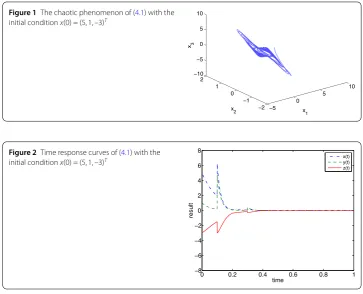
Figure 1The chaotic phenomenon of (4.1) with the initial conditionx(0) = (5, 1, –3)T
Figure 2Time response curves of (4.1) with the initial conditionx(0) = (5, 1, –3)T
In the initial conditionx(0) = (5, 1, –3)T, system (4.1) has chaotic phenomenon when
α= 9.2156, γ= 15.9946, a= –1.24905, b= –0.75735,
as shown in Fig.1. In this case, we can getl= 4.5313.
In order to simplify the calculation, let P=I, τ = 0.1,T = 0.2, ε= 0.5, m= 1, B1= diag(–10, –20, –10),B2= diag(–50, –40, –30), and
Q=
⎡ ⎢ ⎣
3 3 0 0 1 –3 0 0 2
⎤ ⎥ ⎦.
Through simple computation, we getβ1= –10.5898,β2=β3= 1,β4= 8.21,β5= –51.9794,
h1= –1.5272 < 0, h2= –42.9168,η= 36.945, and h1τ +h2(T–τ) +lnη= –0.7630 < 0. So, system (4.1) is exponentially stable by Theorem1 with the initial conditionx(0) = (5, 1, –3)T, as shown in Fig.2.
5 Conclusions
Acknowledgements
The authors would like to express their sincere thanks to referees and the editor for their enthusiastic guidance and help.
Funding
This research is supported by the National Natural Science Foundation of China (Grant Nos. 11561037, 11661047, 11801240).
Availability of data and materials
Not applicable.
Competing interests
The authors declare that they have no competing interests.
Authors’ contributions
The authors contributed equally to the manuscript. Both authors read and approved the final manuscript.
Publisher’s Note
Springer Nature remains neutral with regard to jurisdictional claims in published maps and institutional affiliations.
Received: 19 September 2019 Accepted: 6 November 2019
References
1. Lakshmikantham, V., Bainov, D.D., Simeonov, P.S.: Theory of Impulsive Differential Equations. World Scientific, Singapore (1989)
2. Yang, T.: Impulsive Control Theory. Springer, Berlin (2001)
3. He, W., Meng, T.: Adaptive control of a flexible string system with input hysteresis. IEEE Trans. Control Syst.26, 693–700 (2018)
4. Pan, Y., Yang, G.: A novel event-based fuzzy control approach for continuous-time fuzzy systems. Neurocomputing 338, 55–62 (2019)
5. He, S., Song, J., Liu, F.: Robust finite-time bounded controller design of time-delay conic nonlinear systems using sliding mode control strategy. IEEE Trans. Syst. Man Cybern.48, 1863–1873 (2018)
6. Cardinali, T., Rubbioni, P.: The controllability of an impulsive integro-differential process with nonlocal feedback controls. Appl. Math. Comput.347, 29–39 (2019)
7. Li, X., Song, S.: Stabilization of delay systems: delay-dependent impulsive control. IEEE Trans. Autom. Control62, 406–411 (2017)
8. Xu, H., Teo, K.: Exponential stability with L2-gain condition of nonlinear impulsive switched systems. IEEE Trans. Autom. Control55, 2429–2433 (2010)
9. Huang, T., Li, C., Duan, S., Starzyk, J.A.: Robust exponential stability of uncertain delayed neural networks with stochastic perturbation and impulse effects. IEEE Trans. Neural Netw. Learn. Syst.23, 866–875 (2012)
10. Yang, X., Lu, J.: Finite-time synchronization of coupled networks with Markovian topology and impulsive effects. IEEE Trans. Autom. Control61, 2256–2261 (2016)
11. Lu, J., Ding, C., Lou, J., Cao, J.: Outer synchronization of partially coupled dynamical networks via pinning impulsive controllers. J. Franklin Inst.352, 5024–5041 (2015)
12. Li, X., Ho, D.W.C., Cao, J.: Finite-time stability and settling-time estimation of nonlinear impulsive systems. Automatica 99, 361–368 (2019)
13. Li, X., Yang, X., Huang, T.: Persistence of delayed cooperative models: impulsive control method. Appl. Math. Comput. 342, 130–146 (2019)
14. Sun, J., Zhang, Y., Wu, Q.: Impulsive control for the stabilization and synchronization of Lorenz systems. Phys. Lett. A 298, 153–160 (2002)
15. Zou, L., Peng, Y., Feng, Y., Tu, Z.: Stabilization and synchronization of memristive chaotic circuits by impulsive control. Complexity2017, Article ID 5186714 (2017)
16. Li, C., Feng, G., Liao, X.: Stabilization of nonlinear systems via periodically intermittent control. IEEE Trans. Circuits Syst. II, Express Briefs54, 1019–1023 (2007)
17. Feng, Y., Li, C., Huang, T., Zhao, W.: Alternate control systems. Adv. Differ. Equ.2014, 305 (2014)
18. Hu, X., Nie, L.: Exponential stability of nonlinear systems via alternate control. Ital. J. Pure Appl. Math.40, 671–678 (2018)
19. Horn, R.A., Johnson, C.R.: Matrix Analysis. Cambridge University Press, Cambridge (1985)
20. Zou, L., Peng, Y., Feng, Y., Tu, Z.: Impulsive control of nonlinear systems with impulse time window and bounded gain error. Nonlinear Anal., Model. Control23, 40–49 (2018)