MAC Throughput Improvement Using Adaptive Contention Window

http://dx.doi.org/10.4236/jcc.2015.31001   

MAC

Throughput

Improvement

Using

Adaptive

Contention

Window

Chun‐Liang Lin, Wei‐Ting Chang, Min‐Huei Lu

Department of Electrical Engineering, National Chung Hsing University, Taichung, Taiwan 

Email: 

 

Received 2 January 2015; accepted 19 January 2015; published 23 January 2015 

Copyright © 2015 by authors and Scientific Research Publishing Inc. 

This work is licensed under the Creative Commons Attribution International License (CC BY). 

   

Abstract

HomePlugAV(HPAV)isastandarddevelopedbyHomePlugPowerlineAlliance(HPA)forpower

line communication.InHomePlug AV,it usesatechnologynamedCarrierSenseMultipleAccess

with Collision Avoidance (CSMA/CA) to reduce collisionhappened in network. However, when

networknodes increase,the contentionwindow numbermay notbe wideenough. Itwillcause

collisionprobability toincrease. In thispaper, we introducea newideaof adaptive contention

windowwhichwillproducesuitablecontentionwindowunderactualnetworkenvironment.Our

methodonlyrequirestheinformationofCSMA/CAparameters.Itmeansthatonedoesn’tneedto correcttheoriginalCSMA/CAprocedurebutsubstitutesoldparametersbythenewones.Simula‐

tionexperimentsconductedinthenetworksimulatorNS3showthatcomparedwithHomePlugAV,

ourmethodpromotesthroughputsignificantlywhenthenodenumberincreases.

Keywords

CSMA/CA,ContentionWindow,PowerLineCommunication

1.

Introduction

Power-Line Communication (PLC) is developed rapidly in recent years. Because it doesn’t need to build addi-tional transmit channel and exists almost everywhere even in the backward areas, it is mostly recognized as the solution of “last mile” to the current network communication. Since power line was not originally built for in-formation transmission, there are several problems. One of these is the data collision. When channel transmits multiple packets at the same time, packets will collide naturally causing packets to be destroyed. The station has to retransmit packets which will cause throughput decrease in the end. Thus, HomePlug AV [1] uses CSMA/CA

Although HomePlug AV standard can guarantee high throughput when the number of nodes is very limited, when the node number increases, the value of contention window setting in HomePlug AV will be big which leads throughput to decrease accordingly. In [3], information theory and data mining technique were applied for network traffic profiling. Some research tasks focused on enhancing throughput via the revised MAC layers [3]

[4]-[8]. Among which, the authors of [3] proposed an adaptive contention window mechanism for HomePlug

AV and verified their designs through experiments. They have conducted an experiment to reach the best suc-cessful transmission number in a beacon period. That is, if the number of sucsuc-cessful transmits is less than the optimal one, it means that the current contention window size is inappropriate. It will then change it in the next beacon period. In 2011, the authors of [4] found the optimal contention window value for the situation of dif-ferent nodes. Both of them show that throughput can be improved in an efficient manner if the size of contention window is optimized.

Even though previous research can achieve the desired effect, most of them require information of all stations. That means that they need another bit to transmit that information to each node. Or, they have to modify the protocol. In this research, we propose a new strategy of an adaptive contention window mechanism that doesn’t change the original CSMA/CA procedure or require station’s information as a basis of modifying the contention window size. Our correction factor includes the CSMA/CA parameters. Soft experiments at the network simu-lator, NS3, show the improved effect in throughput.

2.

Principles

of

CSMA/CA

For PLC, when a station tries to send a packet, it first checks the channel condition. If the channel is in idle, it transmits data accordingly. Otherwise, it enters the contention mode. The contention period is a region to con-tend the authority of using channel by other stations.

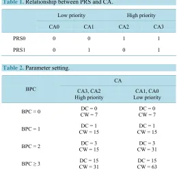
Before going into the contention period, the station will allocate each packet priority. Packets with higher pri-ority use the channel first. If there are several packets possessing the same pripri-ority, it will become the contention period. In priority resolution, HPAV define four parameters, CA0, CA1, CA2 and CA3. CA3 present the highest priority, and CA0 is the lowest, etc. Each station will be defined the packet’s priority in two priority regions de-noted PRS0 and PRS1 respectively. At each PRSi, the station chooses to send or not to send signals. According to the PRS, we can determine the packet’s priority level. Different priority level corresponds to different pa-rameter settings.Table 1 shows the role of it.

After implementing the setting of priority, each station equips with a specific packet priority level. Higher priority level wins the contention and possesses more chances to send the packet. If there are several stations with the same priority, it will proceed to the next stage-random backoff procedure.

For the random backoff procedure, we first introduce contention window and three counters, backoff counter, deferral counter and backoff procedure counter.

1) Contention window (CW): Contention window is a fixed number defined in Table 2. It is used to

deter-mine the value of backoff counters.

2) Backoff counter (BC): Backoff counter’s value chooses from a random value of contention window. It means that CW is the maximal value of BC could be. BC will be decreased by one, each time when it senses a busy status in the channel until BC equals to zero. The station will transmit the packet.

3) Deferral counter (DC): When the number of users in the local area network is large, using only BC to delay the transmission time is not enough. Deferral counter is used to avoid collision further. At the beginning, DC is fixed. Different CAs have different initial values of DC corresponding to. If the channel status sensed is idle, DC remains unchanged. On the contrary, if it is busy, DC will be decreased by one. When DC reaches to zero, the time contention is declared “fail”. It will restart contention again.

[image:3.595.183.442.88.340.2]

Table 1. Relationship between PRS and CA.

Low priority High priority

CA0 CA1 CA2 CA3

PRS0 0 0 1 1

PRS1 0 1 0 1

Table 2. Parameter setting.

CA

BPC _{CA3, CA2}

High priority

CA1, CA0 Low priority

BPC = 0 _{CW = 7} DC = 0 _{CW = 7} DC = 0

BPC = 1 _{CW = 15} DC = 1 _{CW = 15} DC = 1

BPC = 2 _{CW = 15} DC = 3 _{CW = 31} DC = 3

BPC ≥ 3 _{CW = 31} DC = 15 _{CW = 63} DC = 15

fails to transmit packets (happened collision). Station will attempt to contend again and BPC will be increased by one. According to different BPC, there are different DC and CW settings to respond.

We express the behavior through Markov chain [4] inFigure 1. Each time we begin the backoff procedure by

setting the same probability to obtain the value of BC from zero to CW (=W). Therefore, each probability at the top statement is 1/W. At each time slot (defined in HPAV is 35.85 ms), the station will detect the communica-tion channel. The probability is P to sense an “busy”, and it is 1 − P to sense a “idle”. When DC or BC is equal to zero but the channel status sensed is still in busy. BPC will be increased by one and BC will be rechosen. That means that there are too many users occupying the channel. Then, DC and BC need to be increased for longer waiting time for collision avoidance. When BC reaches to zero and the channel status sensed is idle, the station can then transmit packets. The complete flow chart is illustrated inFigure 2.

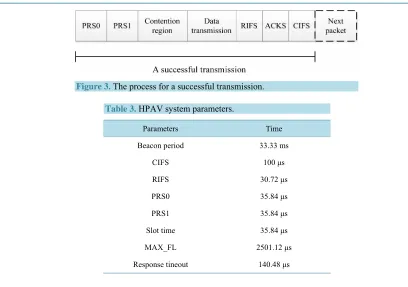
The time of successful transmission can be expressed as inFigure 3. PRS0 and PRS1 are regions to decide

packets priority, a contention region refer to the waiting time of the contended channel before transmitting pack-ets, data transmission is the time of packets sent in the PHY layer; RIFS refers to the time before sending ac-knowledgement, ACK is the time of transmitting acac-knowledgement, and CIFS is time before starting the next packet. Among which, PRS0, PRS1, RIFS, ACKS, and CIFS are fixed numbers in HomePlug AV, seeTable 3.

3.

Slot

Utilization

and

Relation

with

Throughput

Referring toFigure 3, we define r ts

 

and r tc

 

respectively, the time required for a successful data

trans-mission and the time for a collision happened during data transtrans-mission. The two terms can be expressed by

 

all,

 

all

s s c c

r t T  r t T 

where all is the total slot time in the contention region and frame

PRS0 PRS1 RIFS ACK CIFS

s

T   T    (1)

frame

PRS0 PRS1 CIFS

c

T   T  (2) If we define Pb as the probability of slot sensed in busy. From [2], Pb can be expressed by





1 1 n

b

[image:4.595.119.533.85.704.2]

Figure 1. Markov chain of CSMA/CA.

[image:5.595.96.504.75.362.2]

Figure 3. The process for a successful transmission.

Table 3. HPAV system parameters.

Parameters Time

Beacon period 33.33 ms

CIFS 100 μs

RIFS 30.72 μs

PRS0 35.84 μs

PRS1 35.84 μs

Slot time 35.84 μs

MAX_FL 2501.12 μs

Response tineout 140.48 μs

the probability of channel in busy status, it can also be defined as busy slot number

busy slot number idle slot number

b

P 



 ₍₄₎

This is also referred as “slot utilization” [9].

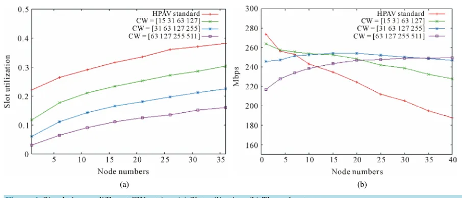
We conduct several extensive simulation experiments on the Network Simulator 3 (NS3) [10]. NS3 is an event driver developed to mimic network environment. Compared with its predecessor NS2, NS3 is completely developed by C++ and the system architecture is simpler than that of NS2. We record slot utilization every 30 seconds at various node arrangement. There are four CW cases in the simulation. The results are shown in Fig-ure 4(a) where Ts defined in Equation (1) is set to be 3500 μs and the slot time is similar to that defined inTable 3.

InFigure 4(a), red line refers to HomePlug AV standard which let CW = [7 15 31 63]. Other lines are the

situation with different CW values. When CW is set to be larger, the probability for obtaining a larger BC is higher. Correspondingly, its slot utilization is comparatively smaller. However, even the CW setting is as such, the slot utilization increases continuously. This fact inspires us to consider whether one can use slot utilization to relate the congestion level. Another simulation been conducted is to observe the variation of throughput at the same setting, illustrated as inFigure 4(b).

InFigure 4(b), HomePlug AV standard has the highest throughput when the number of contention nodes is

small. However, when the node number increases, the throughput will decrease because of the higher collision probability. On the contrary, CW = [63 127 255 511] setting possesses the worst throughput at the beginning. That’s because it wastes too much time in the idle slot. However, it will cause low collision probability when the node number becomes larger. This why it possesses highest throughput when the node number is more than 35.

Therefore, if one can assign the system a low CW setting when the node number is few and a high CW when the node number is large then better throughput could be expected. This is the basic idea behind the adaptive contention window mechanism proposed in this research.

To compareFigure 4(a) andFigure 4(b), from the node number 5 to 12, CW = [15 31 63 127] has the

[image:6.595.84.537.80.274.2]

(a) (b)

Figure 4. Simulation on different CW setting: (a) Slot utilization; (b) Throughput.

In summary, if one can control slot utilization in an appropriate region then better throughput could be ex-pected.

4.

Adaptive

Contention

Window

Mechanism

From [11], it was known that when  defined in Equation (3) as the following way, throughput of the network

will exhibit the best performance:

















.

. .

2 1 1 1 ₁

1 1 2

c avg

c avg c avg

n n T n

n T n T

        

  (5)

where Tc avg. is the average time of collision transmission Tc in the slot time  as

, c

c avg

T T



 (6)

Substituting Equation (6) into Equation (5) yields the new  as

1

2

c

T n





 (7)

Substituting Equation (7) into Equation (3) gives the optimal slot utilization which will lead to the optimal throughput. We set this optimal slot utilization as the standard which is expressed as P_{b opt.} :





. 1 1 1 1

n n

b opt

P

n 

  

     _{ }

  (8)

where 2

c

T  .

After recognized data received, every station records the slot utilization by using Equation (4) for the last successful transmission packet. If slot utilization of the last packet is greater than P_{b opt.} , it means that the cur-rent contention window is not big enough which may cause the congestion. It will assign the system a larger contention window. Otherwise, it will adjust the contention window for reduction. Our adaptive contention window architecture can be illustrated as inFigure 5.

[image:7.595.172.457.85.250.2]

Figure 5. System architecture of the proposed adaptive contention window mechanism.

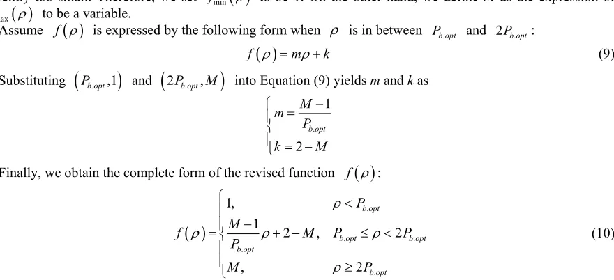
We suppose that the revised function f

 

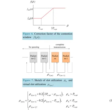
 is given in the form shown inFigure 6. While the slot

utiliza-tion is in between P_{b opt.} and 2P_{b opt.} , f

 

 appears as a linear positive gain. Since CW = [7 15 31 63] is originally suitable for the case with only a few nodes, it doesn’t need to be small when the slot utilization is ap-parently too small. Therefore, we set f_min

 

 to be 1. On the other hand, we define M as the expression of

 

max

f  to be a variable.

Assume f

 

 is expressed by the following form when  is in between P_{b opt.} and 2P_{b opt.} :

 

f  mk (9) Substituting



P_{b opt.} ,1



and



2P_{b opt.} ,M



into Equation (9) yields m and k as

. 1 2 b opt M m P k M         

Finally, we obtain the complete form of the revised function f

 

 :

 

. . . . . 1, 1

2 , 2

, 2

b opt

b opt b opt

b opt

b opt

P M

f M P P

P M P       _           _  (10)

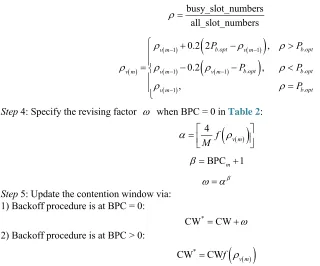
The main idea here is to incorporate slot utilization to determine congestion level of the network. However, slot utilization determined by Equation (4) leads to a large alteration if the last packet is successfully transmitted at BPC = 0 (Table 2). Under this situation, it will bring the next packet with incorrect information in the

con-gestion level. To tackle, we propose a virtual slot utilization instead of the previous slot utilization. A virtual slot utilization will lie in between Pb opt. and 2Pb opt. . The neighboring two packets will not exhibit large difference virtual slot utilization. The virtual slot utilization comes from the following process.

We define _{v m } and _{v m 1} as the virtual slot utilization of the packets m and m1, respectively and m

is the slot utilization of the packet m, shown as inFigure 7.

The packet m + 1 uses _{v m } as the previous slot utilization which adopts Equation (10) to obtain the revising factor as its contention window. _{v m } is obtained by the previous packet’s virtual slot utilization _{v m 1} and the slot utilization of the packet m. If _mP_{b opt.} , _{v m } will be _{ 1} 1



2 _{.  1}



5 b opt

v m P v m

 _   _ to increase the

revising factor. If _mP_{b opt.} , _{v m } will be _{ 1} 1



_{ 1 .}



5 b opt

v m v m P

[image:7.595.98.538.331.532.2]

[image:8.595.152.530.86.457.2]

Figure 6. Correction factor of the contention

window f

 

 .

Figure 7. Sketch of slot utilization _m and virtual slot utilization _{v m }.

   



 



 



 



  . . 1 1 . . 1 1 . 1

0.2 2 ,

0.2 ,

,

b opt m b opt

v m v m

b opt m b opt

v m v m v m

m b opt v m P P P P P                _{  }         < = (11)

By this process, every station CW will reach to a region which the probability of every station transmitting packets will be close. The revising factor f

 

 will be increasing continuously when P_{b opt.} as well.

While the previous method works in an efficient way, there is a weakness, i.e. the contention window mecha-nism shows lower throughput when the node number is few. That’s because if we modify the contention win-dow at BPC = 0 by the previous method, it tends to prompt a larger revising factor when the node number is few. Thus, it still exhibits a large contention window causing lower throughput. It is expected that, at each time in-stant, ρ could really reflect the previous congestion level. Thus, when n is large, we don’t want the station transmits at the first contention period time. It means that one still needs a larger CW at BPC = 0 when the node number is large. Therefore, one has to define an updated revising factor for the state BPC = 0.

Unlike the revising factor characterized inFigure 5 using a simple multiplication to modify the contention

window, the revising factor at BPC = 0 should be updated in the way of addition. Comparing to the multiplica-tion operamultiplica-tion, the amount of addimultiplica-tion should be smaller. It will be more suitable for the case of BPC = 0 since its deferral counter is 0.

The modification is to introduce a correction factor , say

 

 

4 v m f M _{ }  _

  (12)

where the operator

 

 min



n Z n x 



. By this way, we obtain an integer , with its values in between 1 to 4, to indicate the congestion level.

Next, we record the counter of the backoff procedure of the last packet, denoted BPCm. To proceed, set the

BPC_m 1

  

Therefore, the value of  will be from 1 to 4. Combining  and  forms a congestion level indicator as 

 

where Table 4 lists all possible values of .

We choose  as our revising factor when BPC = 0. By this process, the station will has less probability to transmit at the first round in the backoff region when the node number is large. It doesn’t influence throughput when the node number is fewer.

The complete design process of our adaptive contention window process can be summarized as follows: Step 1: Based on the given slot time , collision transmission time T_c and node number n obtain P_{b opt.} as

. 1 2 1 1 b opt c P n T      _ _  

Step 2: Define the revising factor f

 

 by P_{b opt.} :

 

. . . . . 1,

1 _{2 , 2}

,

b opt

b opt b opt

b opt

b opt

P M

f M P P

P M P       _           _ 

Step 3: Count the idle and busy slot numbers of the last transmission packet to obtain the virtual slot utiliza-tion: busy_slot_numbers all_slot_numbers     



 



 



 



  . . 1 1 . . 1 1 . 1

0.2 2 ,

0.2 ,

,

b opt b opt

v m v m

b opt b opt

v m v m v m

b opt v m P P P P P                _{  }   _       

Step 4: Specify the revising factor  when BPC = 0 inTable 2:

 

 

4 v m f M _{ }  _  

BPCm 1

   

  Step 5: Update the contention window via:

1) Backoff procedure is at BPC = 0:

*

CW CW

2) Backoff procedure is at BPC > 0:

 

 

*

CW CWf _{v m}

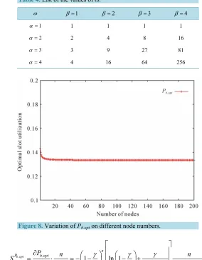
So far, our focus is only in own station. However, the station number in Equation (8) is not fixed which is unknown in general. To resolve this problem, we calculate Pb.opt



Tc3500 s



with different n, seeFigure 8.

When the node number is in 1 ~ 200, its value will not significantly affect P_{b opt.} . To prove the node numbers will not influence P_{b opt.} further, we calculate the sensitivity when n is larger than 200.

Define 2

c

T



[image:9.595.96.416.369.635.2]

4

[image:10.595.91.477.80.618.2]

 4 16 64 256

Figure 8. Variation of Pb.opt on different node numbers.

. .

.

1 ln 1

1 _{1 1}

b opt

n P b opt

n n

b opt

P n n

S

n P n n

n n _n     _      _{   }       _{  }  _       _{ } _ _{ }   _{ }      

When n > 200, the terms 1

n

n 

 _   

  and

1 1 n n n     _{ }  

will be smaller than 1. However,

ln 1 1

1 n n n     _ _   _{ }   _    

 . Thus, S0.

In the following study, the network node number n is set to be 10. Furthermore, if we consider CW = [127 255 511 1023] as the largest contention window, which will be approximately 15 times to the case of CW = [7 15 31 63], then we set the maximum revising function M to be 15.

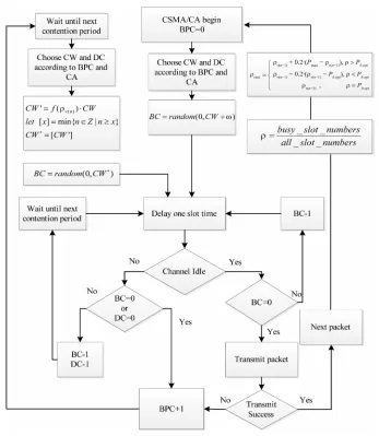
The operational flow chart of the updated adaptive contention window mechanism is illustrated inFigure 9.

5.

Experimental

Results

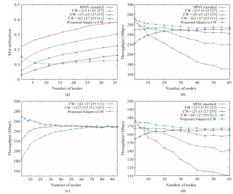
The goal of this research is to acquire higher throughput while maintaining slot utilization. The simulation ex-periments have been conducted at the network simulator NS3. We set  to be 35.84 μs which remains the same as in HomePlug AV. Simulation study is mainly conducted for different Ts and CW.

Figure 10(a)shows slot utilization for various CW settings. No matter HomePlug AV standard or other CW

[image:10.595.161.445.91.455.2]

[image:11.595.138.485.79.478.2]

Figure 9. Operational flow chart of the proposed adaptive CW mechanism.

only slight difference among different cases in our proposed approach. This result shows that our method is ef-fectively to control slot utilization. Even for a large scale network, it shows no significant difference.

After verifying slot utilization, the main point of this research is to get better throughput on the large scale network.

We prove in the follows that the proposed approach exhibits the best throughput performance while compar-ing to other fixed CW settcompar-ings.

Including the original HomePlug AV (CW = [7 15 31 63]). All packets are supposed to possess the same pri-ority and all stations are on the saturated situation which means that all stations have packets to transmit at all time. We record the average throughput every 30 seconds for each condition.

Figure 10(b)shows throughput of various CW settings with Ts equal to 3500 μs. HomePlug AV standard

(a) (b)

[image:12.595.72.534.79.464.2]

(c) (d)

Figure 10. Various CW settings in different simulation cases: (a) Slot utilization; (b) Throughput (Ts = 3500 μs); (c)

Throughput (large node number and large CW); (d) Throughput (Ts = 5500 μs).

number is increased to 95, it performs as the cases of CW = [127 255 511 1023] in the simulation study. The simulation result shows that when the node number approaches to a large value, throughput will converge to a small region. Thus, setting an extremely large CW doesn’t bring positive effect. That’s also the reason that we set a limit to f

 

 .

To prove performance robustness of the present mechanism, we conduct experiments for different transmis-sion time. Figure 10(d) illustrates that throughput of the successful transmission time equals 5500 μs. This

shows the similar result, our method performs the best at all time. FromFigure 10(b) andFigure 10(d), it can

be seen that if transmission time is less, the degree of CW affecting throughput is larger and our adaptive CW mechanism performs better than other cases as well.

We also verify the case when there is an abrupt change in the node number and examine if it still works. Con-sider the network has 40 nodes at the beginning. At 60 seconds, it reduces to 10 nodes. We compare the situation with 10 nodes at the beginning and record throughput at each second. The simulation result is shown inFigure 11(a). It displays that after 60 seconds, throughput of the situation 1 has been improved and quickly approaches

to the line of situation 2. This endorses performance robustness of our proposed mechanism

Finally, the number n in Equation (8) was changed to 10 at the previous simulation test. To prove that it won’t significantly alter the result, we conduct extra tests with the number of nodes n = 30 and compare it to the case of n = 10. SeeFigure 11(b) for the result. It clearly shows that the value of n doesn’t significantly affect

[image:13.595.76.533.81.264.2]

(a) (b)

Figure 11. Throughput at different special case: (a) Situation 1: 40 nodes at network beginning. It remains 10 nodes after 10 s. Situa-tion 2: 10 nodes at all time; (b) Various setting of Pb.opt.

6.

Conclusion

PLC is becoming mature in recent years. However, as the usual network communication, the network conges-tion problem is crucial when considering maintaining communicaconges-tion quality. While HomePlug AV is already a mature protocol in PLC, we propose here an adaptive contention mechanism instead of formulating a new pro-tocol. The adaptive contention window scheme only needs the information from CSMA/CA in HomePlug AV. In addition, because the information needed is self-contained, one does not need not to correct the PHY layer setting to acquire extra information from other stations. All needed are to substitute the new CW and BC into the original HomePlug AV mechanism. This makes the approach more practical and presents better feasibility. From the simulation experiments conducted at NS3, it is found that the proposed scheme can effectively im-prove throughput. We have tested it with a variety of several scenarios; satisfactory results have been observed which show identifiable improvement of our proposed design.

Acknowledgements

This research was sponsored by National Science Council, Taiwan, under the Grant NSC 101-2221-E-005- 015-MY3.

References

[1] HomePlugPowerline Alliance (2007) HomePlug AV Specification, Ver. 1.1.

[2] Chung, M.Y., Jung, M.H., Lee, T.J. and Lee, Y. (2006) Performance Analysis of HomePlug 1.0 MAC with CSMA/CA.

IEEE Journal on Selected Areas in Communications, 24, 1411-142

[3] Velarde-Alvarado, P., Martinez-Pelaez, R., Ruiz-Ibarra, J. and Morales-Rocha, V. (2014) Information Theory and

Da-ta-Mining Techniques for Network Traffic Profiling for Intrusion Detection. Journal of Computer and

Communica-tions, 2, 24-30

[4] Yoon, S.G. and Bahk, S. (2011) Adaptive Rate Control and Contention Window-Size Adjustment for Power-Line

Communication. IEEE Transactions on Power Delivery, 26, 809-816.

[5] Kriminger, E. and Latchman, H. (2011) Markov Chain Model of HomePlug CSMA MAC for Determining Optimal

Fixed Contention Window Size. Proceedings of IEEE International Symposium on Power Line Communications and

Its Applications, Udine, 3-6 April 2011, 399-404.

[6] Liu, K.H., Hsieh, D.R., Hsu, J.Y. and Chang, S.Y. (2012) Throughput Improvement for Power Line Communication by

Adaptive MAC Protocol. Proceedings of IEEE International Power Engineering and Optimization Conference,

Me-laka, 6-7 June 2012, 135-140.

Proceed-[11] Bianchi, G. (2000) Performance Analysis of the IEEE 802.11 Distributed Coordination Function. IEEE Journal on