Munich Personal RePEc Archive
Time series properties of ARCH
processes with persistent covariates
Han, Heejoon and Park, Joon Y.
May 2006
Online at
https://mpra.ub.uni-muenchen.de/5199/
Time Series Properties of ARCH Processes with
Persistent Covariates *
Heejoon Han and Joon Y. Park
RMI Working Paper No. 06/11
Submitted: December 5, 2006
Abstract
We consider ARCH processes with persistent covariates and provide asymptotic theories that
explain how such covariates affect various characteristics of volatility. Specifically, we
propose and study a volatility model, named ARCH-NNH model, that is an ARCH(1) process
with a nonlinear function of a persistent, integrated or nearly integrated, explanatory variable.
Statistical properties of time series given by this model are investigated for various volatility
functions. It is shown that our model generates time series that have two prominent
characteristics: high degree of volatility persistence and leptokurtosis. Due to persistent
covariates, the time series generated by our model has the long memory property in volatility
that is commonly observed in high frequency speculative returns. On the other hand, the
sample kurtosis of the time series generated by our model either diverges or has a
well-defined limiting distribution with support truncated on the left by the kurtosis of the
innovation, which successfully explains the empirical finding of leptokurtosis in financial
time series. We present two empirical applications of our model. It is shown that the default
premium (the yield spread between Baa and Aaa corporate bonds) predicts stock return
volatility, and the interest rate differential between two countries accounts for exchange rate
return volatility. The forecast evaluation shows that our model generally performs better than
GARCH(1,1) and FIGARCH at relatively lower frequencies.
Keywords: ARCH, nonstationarity, nonlinearity, NNH, volatility persistence, leptokurtosis.
Heejoon Han
Department of Economics
National University of Singapore
5 Arts Link, AS2 04-36
Singapore 117570
Tel: (65) 65166258
Fax: (65) 6775 2646
E-mail:
[email protected]
Joon Y. Park
Department of Economics
Texas A&M University
Allen 3084
4228 TAMU, College Station
TX 77843
Tel: (979) 845-7309
E-mail:
[email protected]
1
Introduction
ARCH type models have widely been used to model the volatility of economic and …nancial time series since the seminal work by Engle (1982) and the extension made by Bollerslev (1986). The processes generated by these models successfully show volatility clustering and leptokurtosis, which are commonly observed for many economic and …nancial time series. However, most of the volatility characteristics of these models have been univariate, relating the volatility of time series only to the information contained in its own past history. Hence, they shed little light on a source of volatility and exclude the possibility that conditional heteroskedasticity may be accounted for by some economic variables.
As an e¤ort to provide some structural or economic explanations for volatility, many pre-vious works considered ARCH type models with exogenous variables. Typically, GARCH(1,1) model with an exogenous variable (mostly in linear form) was used for this purpose. En-gle and Patton (2001) tested a GARCH(1,1) model with three month U.S. Treasury bill rates for stock return volatility, and Gray (1996) added the level of interest rates to explain conditional variance in his generalized regime-switching model of short-term interest rates. Likewise, forward-spot spreads and interest rate di¤erentials between countries were used as covariates respectively by Hodrick (1989) and Hagiwara and Herce (1999) to model ex-change rate return volatility. Moreover, Lamoureux and Lastrapes (1990) included trading volumes in their stock return volatility model.
The exogenous variables such as interest rates and interest rate di¤erentials between countries used in these works are known to be highly persistent, and may well be mod-eled as time series having an exact or near unit root. It is therefore natural to expect the persistent covariates would a¤ect the degree of persistence in volatility. However, there has been no theoretical study in the literature to rigorously investigate the e¤ects of the presence of persistent covariates on volatility persistence. They have been largely ignored, and researchers usually focus on the ARCH e¤ects to analyze the degree of volatility persis-tence. The main motivation of our research is to …ll this gap, by providing some important asymptotic theories for ARCH models with persistent covariates. In particular, our theories make it clear how persistent covariates a¤ect volatility persistence and leptokurtosis.
Recently, Park (2002) introduced nonstationary nonlinear heteroskedasticity (NNH). NNH models specify conditional variance of given time series as a nonlinear function of an integrated process. The function generating conditional heterogeneity is called heterogene-ity generating function (HGF). It is shown that volatility clustering and leptokurtosis are manifest for NNH models and, in contrast, stationary nonlinear heteroskedasticity (SNH)2 does not produce volatility clustering.
We introduce a volatility model which combines an ARCH(1) model with the NNH model. We call this model ARCH-NNH. Unlike Park (2002), we allow the NNH part of our models to be generated by a covariate which has a near unit root as well as an exact unit root. Therefore, our models represent a wide class of time series with volatilities
2In contrast to the NNH model, the conditional heterogeneity is generated by a stationary process in the
driven by the autoregression with persistent covariates. The statistical properties of ARCH-NNH models depend crucially on the type of HGF. Two di¤erent classes of functions are considered: integrable (f 2I)andasymptotically homogeneous (f 2H)functions, following Park and Phillips (1999, 2001) who introduced them in their studies on nonlinear models with integrated time series.
We investigate various statistical properties of time series driven by ARCH-NNH mod-els. The asymptotic behavior of sample autocorrelation of squared process generated by ARCH-NNH models shows that volatility clustering is expected for ARCH-NNH models with various HGF’s; the autocorrelation is very persistent, i.e., they vanish very slowly or do not even vanish for all lags.
Ding et al (1993) found that it is possible to characterize the power transformation of stock return to be long memory. The sample autocorrelation function of squared speculative returns (especially high frequency data) is known to have a typical trend that it decreases fast at …rst and remains signi…cantly positive for larger lags. The fractionally integrated models such as Long Memory ARCH model by Ding and Granger (1996) and FIGARCH model by Baillieet al (1996) are known to capture this long memory property in volatility. Recently, several studies have shown that a number of nonlinear short memory volatility models can also produce spurious long memory characteristics in volatility. One example of such models is the volatility component model by Engle and Lee (1999). And theoretical works in structural change (Mikosch and Starica (2004)), switching regime (Diebold and Inoue (2001)), and occasional breaks (Granger and Hyung (2004)) have shown that any of these events is capable of producing the long memory property.
Our theory shows that ARCH-NNH can also generate the long memory property in volatility. Asymptotically, the autocorrelation function of squared process of ARCH-NNH model with f 2 I decreases to zero at a hyperbolic rate as the lag order increases. While the autocorrelation function of squared process of GARCH (1,1) vanishes at an exponential rate, that of ARCH-NNH model does at a hyperbolic rate like the fractionally integrated models. On the other hand, the asymptotic autocorrelation function of squared process of ARCH-NNH model with f 2H decreases fast (exponentially) at …rst and converges to some positive random limit. Regardless of the function class of HGF, ARCH-NNH models generate the long memory property in volatility due to persistent covariates.
Similarly as those for the volatility component model by Engle and Lee (1999), the time series generated by ARCH-NNH models can be decomposed into the permanent or long-run component (NNH term) and the transitory or short-long-run (ARCH term) component. Only a shock to the persistent covariates has a long-run e¤ect on volatility. Additionally, we compare the autocorrelation functions of simulated ARCH-NNH, GARCH(1,1), and FIGARCH processes, which shows that ARCH-NNH processes mimic the movement of real data very well.
Time series generated by ARCH-NNH models with various HGF’s all unambiguously predict the presence of leptokurtosis. The sample kurtosis of ARCH-NNH models with
f 2Idiverges at the rate ofpn, which means it is expected to have a large sample kurtosis for any reasonably large sample. The sample kurtosis of ARCH-NNH models with f 2H
simple power function. One is a stock return volatility model and the persistent covariate used for the model is the default premium (the yield spread between Baa and Aaa corporate bonds). It shows that stock return volatility is well explained by the default premium, which con…rms the earlier work by Schwert (1989). The other application is the model for exchange rate return volatility, where we use as a covariate the interest rate di¤erentials between two countries. We could see the modulus of the interest rate di¤erential is well explaining exchange rate return volatility, as observed by Hagiwara and Herce (1999). In both cases, the ARCH-NNH model appears to be quite appropriate and this indicates that the default premium is a proper source of stock return volatility and the interest rate di¤erential is an adequate source of exchange rate return volatility.
Finally, we evaluate the forecasting ability of the ARCH-NNH model. We obtained out-of-sample forecasts at the monthly, weekly and daily frequencies. Using ‘realized volatility’ as a proxy for actual volatility, we employ the regression-based method and the mean ab-solute error with the forecast accuracy tests by Diebold and Mariano (1995). It is shown that the ARCH-NNH model is not only practically useful, but also outperforms GARCH(1,1) and FIGARCH at relatively lower frequencies.
The rest of the paper is organized as follows. Section 2 introduces the model with some preliminary concepts. Various statistical properties for the samples from ARCH-NNH models are investigated in Section 3. The asymptotic behavior of sample statistics such as sample autocorrelation of squared process, as well as sample variance and kurtosis, is derived. Section 4 presents empirical applications of ARCH-NNH model. The forecasting ability of ARCH-NNH model is evaluated in Section 5. Section 6 concludes the paper, and Appendices A and B contain mathematical proofs for the technical results in the paper.
2
The Model and Preliminaries
We write our volatility model as
yt= t"t (1)
and let (Ft) be a …ltration, denoting information available at time t.
Assumption 1 Assume that
(a) ("t) is iid (0,1) and adapted to (Ft)
(b) ( t) is adapted to (Ft 1)
Under assumption 1, we have
E(ytjFt 1) = 0 and E(yt2jFt 1) = 2t:
The time series(yt)has conditional mean zero with respect to the …ltration (Ft), and
there-fore, (yt;Ft) is a martingale di¤erence sequence. However, it is conditionally heteroskedastic
Assumption 2 Let
2
t = yt2 1+f(xt) (2)
for some nonnegative functionf :R!R+and
xt= 1 c
n xt 1+vt (3)
assuming that (xt)is adapted to (Ft 1) wherec 0:
Assumption 1 and 2 de…ne our volatility model. Under Assumption 1 and 2, (yt) is
an ARCH process with persistent covariates. The volatility model given by 2t = f(xt) is referred to as Nonstationary Nonlinear Heteroskedasticity (NNH), which is introduced by Park (2002). Park (2002) considered only the case in which(xt)has an exact unit root. We
add this NNH term in our volatility model with an extension that allows(xt)to have anear unit root as well. The speci…cation in (3) allows that (xt) has not only an exact unit root
but also a near unit root. Since our volatility model is a combination of ARCH(1) and NNH models, it will be referred to as ARCH-NNH in our subsequent discussions. Notice that our model does not include 2t 1 term:Our theory will show that this term is not necessary and instead persistent covariates mainly explain volatility persistence.
The function f :R!R+will be referred to asheterogeneity generating function(HGF) in what follows. Clearly, f must be a nonlinear function, since it has to be nonnegative. More speci…cally, we consider two classes of functions: integrable andasymptotically homo-geneous functions. These function classes were introduced by Park and Phillips (1999) in their study on the asymptotics of nonlinear transformations of integrated time series. As it was done by Park (2002), the functions that are integrable and asymptotically homoge-neous will be calledIandH-regular with added regularity conditions. They will be denoted respectively by I and H.
To derive the asymptotics for the ARCH-NNH models with f 2I, we assume that(vt)
in (3) is either iid sequence with Ejvtjq < 1 for some q > 4 (as in Assumption 3S), or a stationary linear process driven by an iid sequence ( t) such that Ej tjq < 1 for some
q >4 (as in Assumption 4S). In the following de…nition, we let q be the number that will be given later by such moment conditions.
De…nition 2.1 A transformation f on R is called I-regular (f 2 I) if f is bounded, integrable and piecewise Lipschitz, i.e.,
jf(x) f(y)j cjx yj`
on each piece of its support, for some constantc and` >6=(q 2):
To de…neH-regular functions, we introduce some classes of transformations onR:We denote byzB the class of all bounded transformations onR;and denote byzLB the class of locally bounded transformations on R: De…ne z0B be the class of all bounded functions vanishing at in…nity, and letz0LB be the subset ofzLB consisting ofT such thatT(x) =O(exp(cjxj))
De…nition 2.2 A transformation f on R is calledH-regular (f 2H) iff can be written as
f( x) = ( )f(x) +R(x; )
for large uniformly inxover any compact interval, wheref is locally Riemann integrable and R satis…es
R(x; ) =a( )p(x) or b( )p(x)q( x)
with a and b such that a( )= ( ) ! 0 and b( )= ( ) < 1 as ! 1;and p and q such that p2z0LB and q 2zB0:For f 2H, We call and f ; respectively, the asymptotic order and limit homogeneous function of f:
The reader is referred to Park and Phillips (1999, 2001) for more details on these function classes. The classesIandHinclude a wide class, if not all, of transformations de…ned onR. The bounded functions with compact supports and more generally all bounded integrable functions with fast enough decaying rates, for instance, belong to the classI . On the other hand, power functions ajxjb with b 0 belong to the class H having asymptotic order
a b and jxtjb as limit homogeneous functions. Moreover, logistic function ex=(1 +ex) and
all the other distribution function-like functions are also the elements of the class H with asymptotic order 1 and limit homogeneous function 1fx 0g:
Standard terminologies and notations in probability and measure theory are used through-out the paper. In particular, notations for various convergences such as !a:s:;!p and!d
frequently appear. The notation =d signi…es equality in distribution. Some theoretic tools
are introduced in the following. In the next section, we are going to introduce assumptions for(vt);which make the time series(xt)in (3) become a general linear process with a near
unit root or an exact unit root. Throughout the paper, we set the long-run variance of(vt)
to be unity because it has only an unimportant scaling e¤ect on our analysis. Either As-sumption 3 or AsAs-sumption 4 in the next section satis…es conditions of(vt)for the followings.
We de…ne
Vcn(r) =n 1=2x[nr]
forr2[0;1];where[z]denotes the largest integer which does not exceedz:And we let
Vc(r) =
Z r
0
exp ( c(r s))dV0(s)
wherer 2[0;1]and V0 is the standard Brownian Motion. Then, it is well known that
Vcn!dVc
as n ! 1: Vc is an Ornstein-Uhlenbeck process, generated by the stochastic di¤erential
equation
dVc(r) = cVc(r)dr+dV0(r)
As in Park (2003), our subsequent theory for the case of integrable HGFs involves the local time of Ornstein-Uhlenbeck process. The local time forVc is then de…ned as
Lc(t; s) = lim "!0
1 2"
Z t
0
1fjVc(r) sj< "gdr:
Roughly speaking,2"timesLc(t; s)measures the actual time spent byVcin the"-neighborhood
of sup to time t: The local time yields theoccupation time formula
Z t
0
T(Vc(r))dr= Z 1
1
T(s)Lc(t; s)ds
for any T : R!R locally integrable. For each t; the occupation time formula allows us to evaluate the time integral of a nonlinear function of an Ornstein-Uhlenbeck process by means of the integral of the function itself weighted by the local time.
3
Statistical Properties of ARCH-NNH
We investigate the statistical properties of ARCH-NNH models. In particular, the asymp-totic behavior of the sample autocorrelation function of squared process and other sample moments such as sample variance and sample kurtosis of process generated by ARCH-NNH models are derived.
3.1 Sample Autocorrelation of Squared Process
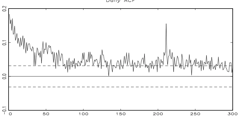
Dinget al (1993) investigated the long memory property of stock returns and they found out that it is possible to characterize the power transformation of stock returns to be long mem-ory. This long memory property is known to be commonly observed in high frequency data. Figure 1 shows the sample autocorrelation function of daily squared returns on S&P 500 in-dex and this con…rms the long memory property; the autocorrelation function decreases fast at …rst and remains signi…cantly positive for larger lags. Hitherto the fractionally integrated models such as Long Memory ARCH model by Ding and Granger (1996) and FIGARCH model by Baillieet al (1996) are known to capture this property.
De…ne the sample autocorrelation of (yt2) by
R2nk =
n P
t=k+1
y2
t yn2 yt k2 y2n n
P t=1
y2
t yn2
2 ;
wherey2
ndenotes the sample mean of(y2t):To precisely characterize the asymptotic behavior
of R2nk under ARCH-NNH models, we make the following additional assumptions.
Assumption 3S Assume (a)(vt) are iid.
(b)Ef2(x+vkt)<1 for all x2Rand k 1, wherevkt=vt+1+:::+vt+k:
(c)Ej"tjp <1 for somep 8:
(d)("t)and (vt) are independent.
(e) (vt) has distribution absolutely continuous with respect to Lebesgue measure,
charac-teristic function (t) such thattr (t) ! 0 as t ! 1 for some r > 0, and Ejv
tjq <1 for
someq >4:
Assumption 3W Assume (a)-(e) of Assumption 3S withq >2:
Assumption 3W is weaker than Assumption 3S, where ‘W’ and ‘S’ stand for weak and strong respectively. Whenever the distinction is unnecessary, we will just refer to Assump-tion 3. Under AssumpAssump-tion 3S, (vkt) has density with respect to Lebesgue measure on R,
and we signify the density bypk:Also, we denote the kurtosis of ("t) by 4" throughout the paper.
Theorem 1 Let Assumptions 1 and 2 hold, and let k 1: Assume that 0 < < 1 and
2 4
" <1:
(a) If f 2I, then under Assumption 3S
R2nk !p
1
Z
1 1
Z
1
f(x)f(x+y)kP1
j=0 1
P i=0
i+jp
k+i j(y)dxdy
2 4
"
1 2 4
"
1
Z
1 1
Z
1
f(x)f(x+y)P1
i=1
ip
i(y)dxdy+
4
"
1 2 4
"
1
Z
1
f2(s)ds
+ k
as n! 1:
(b) If f 2H with limit homogeneous function f, then under Assumption 3W
R2nk !d
(1 k) R1
0 f2(Vc(r))dr
R1
0 f(Vc(r))dr 2
(1 2)
1 2 4
"
4
" R1
0 f2(Vc(r))dr
R1
0 f(Vc(r))dr
as n! 1:
Theorem 1 shows the asymptotic behavior of the sample autocorrelations of squared process generated by ARCH-NNH models. Regardless of function classes, probability limits of R2nk contain k: Considering that R2nk of ARCH(1) converges to k, we can tell that
k term comes from the ARCH component and the other term of each case is originated
from the NNH component. (Recall that ARCH-NNH model is a combination of ARCH(1) and NNH.) In the following context, we can see that persistent covariates mainly explain volatility persistence and also generate the long memory property in volatility.
The part (a) of Theorem 1 shows that, for ARCH-NNH models withf 2I,R2nkconverges in probability to a nonrandom limit, which as a function of k 1 we may regard as the asymptotic autocorrelation function of squared process and we denote R2
k hereafter. The
actual value of R2k is determined by the distribution of (vt) as well as HGF. In order to explain volatility persistence, R2k should at lease decrease at a slow rate as k ! 1: As it was done by Park (2002), let us consider the case in which the distribution of (vt) is
Gaussian. Since we havevkt =d
p
kvt in the case, it follows thatpk(x) = p1kp pxk where p is the normal density. Since the normal density is continuous at the origin, we have
1 Z 1 1 Z 1
f(x)f(x+y)pk(y)dxdy =
1 p k 1 Z 1 1 Z 1
f(x)f(x+y)p(py
k)dxdy
= p1
kp(0) 0
@
1
Z
1
f(x)dx 1
A
2
!0
ask! 1:
Using this, we can show that R2
k in part (a) of Theorem 1 decreases to zero ask! 1:
When (vt) is Gaussian, we have
k 1 X j=0 1 X i=0
i+jp
k+i j(y) = k 1
X
j=0
jX1 i=0
ip 1 k+i jp(
y
p
k+i j):
Letc be an arbitrary number such that0< c < k 1:Forj=c;as k! 1 j
1
X
i=0
ip 1 k+i jp(
y
p
k+i j)!0
because p 1
k+i j will dominate and the rate of decay is k
1=2. Forj =k c; then j will
dominate and we have an exponential convergence rate. Sincecis arbitrary, we can divide
kP1
j=0
j P1 i=0
ip 1
k+i jp( y
p
k+i j)into two parts; one part decays at a hyperbolic ratek
1=2 and
the other part does at an exponential rate k. So, we can deduce that
k 1
X
j=0
jX1 i=0
ip 1 k+i jp(
y
p
ask! 1and its decay rate is hyperbolic. The fact that R2
k converges to zero is similar with the behavior of GARCH(1,1) model.
However, there is an important di¤erence in their respective decreasing patterns. Under GARCH(1,1),R2k decreases at an exponential rate ask increases.3 However, R2k of ARCH-NNH models withf 2Idecreases at a hyperbolic rate. This means that ARCH-NNH models with f 2 I produce the long memory property in volatility as the fractionally integrated models do. In other words, volatility persistence is well expected in ARCH-NNH models withf 2I.
On the other hand, the part (b) of Theorem 1 gives the asymptotic limit of R2nk for ARCH-NNH models with f 2 H; and it is very di¤erent from that of the previous f 2 I
case. Since an Ornstein-Uhlenbeck process is included,R2
k is random and it is not a¤ected
by the distribution of (vt): Rk2 of ARCH-NNH models withf 2H decreases ask! 1but it does not converge to zero. Let
A=
1 (1 )
R1
0 f2(V(r))dr
R1
0 f(V(r))dr 2
(1+ ) 4
"
1 2 4
"
R1
0 f2(V(r))dr (11 )
R1
0 f(V(r))dr 2:
Then,
R2k=A+ k(1 A):
Ask! 1; R2kdecreases exponentially at …rst and …nally converges toAwhich is a random constant clearly smaller than unity and positive unless limit homogeneous function f is constant. This trend of R2k is compatible with the sample autocorrelation of the real data in Figure 1. Like the previousf 2I case, ARCH-NNH models withf 2Halso capture the long memory property in volatility. Therefore, it is also expected that ARCH-NNH models withf 2Hwould properly explain volatility persistence.
When f 2 H, Rk2 of ARCH-NNH models behaves similarly as that of NNH models. However,R2
kof ARCH-NNH models withf 2His dependent onkand decreases ask! 1;
which is di¤erent from R2k of NNH models. In case of NNH models with f 2 H, R2k is independent ofk and given by a random constant for all values of the lag orderk 1:
Additionally, the result in part (b) of Theorem 1 implies that if f has constant limit homogeneous functions then the sample autocorrelation of squared process by ARCH-NNH models converges in probability to k:Suppose that f(xt) =c+g(xt) where c is constant
and g(xt)2I. Then f is asymptotically homogeneous and its limit homogeneous function
is constant. This means R2nk !p k just like ARCH(1). Note that if an ARCH-NNH
model hasf(xt) =c then it is exactly the ARCH(1) model. Therefore, iff(xt) consists of
constant and g(xt) 2 I, the integrable function g(xt) does not a¤ect volatility persistence
asymptotically.
Theorem 1 shows that, due to persistent covariates, ARCH-NNH process explains volatil-ity persistence very well and, especially, produces the long memory property in volatilvolatil-ity.
3The sample autocorrelation of the squared process of stationary GARCH(1,1) has probability limit given
by ( + )k 1 (1 2)
1 2 2 for k 1if
2 4
The following text gives us better understanding about how persistent covariates play a role in volatility persistence.
3.1.1 Decomposition of Volatility
In the volatility component model by Engle and Lee (1999), volatility is decomposed into a permanent or long-run component and a transitory or short-run component. Similarly, an ARCH-NNH model has two components, and an NNH term represents a permanent/long-run component while an ARCH term explains a transitory/short-permanent/long-run component. We follow the way done by Ding and Granger (1996), who showed that, for the IARCH(1) process, a shock may permanently a¤ect the ‘expectation’ of a future conditional variance process, but it does not permanently a¤ect the ‘true’ conditional process itself.
According to assumption 2, xtis adapted to (Ft 1). To make it simple, let us consider
the case in which xt is adapted to (Ft), "t N(0;1)and @f@x(x) 6= 0. Then we have
yt = t"t; "t N(0;1) (4)
2
t = yt2 1+f(xt 1) (5)
xt = 1 c
n xt 1+vt (6)
In ARCH-NNH models, a shock to the system at time t comes from "t orvt;and this
shock will not a¤ect 2t because 2t depends only on the past information. Since
2
t+k= kY1
i=1
"2t+k i ky2t +
k 1
X
j=0
j Y
i=1
"2t+k i jf(xt+k 1 j)
(we let Q0
i=1
"2t+k i = 1 here), we have
E(yt2+k) =E( 2t+k) = kyt2+ k 1f(xt) + k 2
X
j=0
jE(f(x
t+k 1 j)):
A shock at time t to y2t; from "t; and a shock to xt, from vt; will permanently change
E(yt2+k) andE( 2t+k);i.e., both shocks a¤ect the ‘expectation’ of the future squared process and the future conditional variance process. However, we have di¤erent situation in case of the ‘true’ y2t+k and 2t+k:The real impact of a shock from"t (a change inyt2) to 2t+k is
@ 2t+k @yt2 =
kY1
i=1
and the real impact of a shock fromvt (a change inxt) to 2t+k is
@ 2t+k @xt
=
k 1
X
j=0
j Y
i=1
"2t+k i j@f(xt+k 1 j) @xt
=
k 1
X
j=0
j Y
i=1
"2t+k i j 1 c
n
k 1 j @f(xt+k 1 j) @xt+k 1 j
because @f(xt+k 1 j)
@xt =
@f(xt+k 1 j)
@xt+k 1 j
@xt+k 1 j
@xt =
@f(xt+k 1 j)
@xt+k 1 j 1
c n
k 1 j :
Corollary 2 Given (4)-(6), let k 1, 0< 1, and @f@x(x) 6= 0: As k! 1;
(a) @ 2t+k
@y2
t !a:s:0.
(b) @ 2t+k
@xt !a:s:h for some h >0 if c= 0:
(c) @ 2t+k
@xt !0 at a slower rate than
@ 2
t+k
@y2
t if c >0 and
2 4
" <1:
Note in the part (a) of Corollary 2 that even if = 1; @ 2t+k
@y2
t ! 0 almost surely as
k ! 1. This is because, as shown in Nelson (1990), kQ1
i=1
"2
t+k i in (7) converges to zero
almost surely. Similarly, it should be noticed that the part (b) of Corollary 2 holds even when = 1: Since yt2+k = 2t+k"2t+k; we have the similar result for yt2+k. Therefore, the part (a) and (b) of Corollary 2 indicate that while the real impact of a shock from "t will
converge to zero, a shock tovtwill permanently a¤ect the ‘true’ process of 2t+k andyt2+kif
xt is an I(1)process. A shock to "t is not persistent in 2t+k and yt2+k, but a shock tovt is
persistent in 2
t+kand yt2+k:Ifc >0;then the real impact of a shock fromvt will disappear
eventually. However, the part (c) of Corollary 2 shows that a shock from vt has a longer
e¤ect than a shock from "t. Hence, we can consider a shock from "t as a short-run shock
and a shock fromvt as a long-run shock.
3.1.2 Simulated Autocorrelation Functions
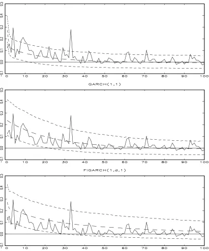
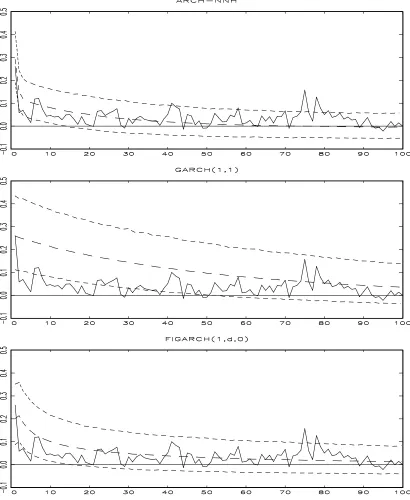
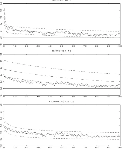
We generated data using the estimates obtained from our …rst empirical application in the section 4 and drew autocorrelation functions for the ARCH-NNH model with a simple power function, GARCH (1,1) model and FIGARCH(1,d,q)4 model based on 5;000
iteration. The upper and lower dotted curves indicate the 5%- and 95%-quantile of the distribution of the autocorrelations at a …xed lag and the middle dotted curves correspond to the mean of those distributions.
Overall, the simulations show that ARCH-NNH processes mimic the movements of the real data very well. For the monthly case, the simulated ARCH-NNH process performs very well in following the movement of the real data. Even if GARCH(1,1) and FIGARCH are also doing …ne, their simulated processes are a little higher than the autocorrelation function of the real data. For the weekly and daily cases, both our model and FIGARCH are doing well, but it is obvious that GARCH(1,1) is not proper in following the movement of the real data.
3.2 Sample Variance and Kurtosis
We now investigate the asymptotic behaviors of other sample moments such as sample variance and kurtosis. The sample variance of (yt)is de…ned by
S2n= 1
n n X
t=1
yt2:
We introduce additional assumptions for the asymptotics of the sample variance.
Assumption 4S Assume (a)Ej"tjp <1 for somep 4:
(b)(vt) is generated by
vt= (L) t=
1
X
k=0
k t k (8)
where 0 = 1; (1) 6= 0 with
X1
k=0kj kj < 1, and ( t) are iid and has distribution
absolutely continuous with respect to Lebesgue measure, characteristic function '(t) such thattr'(t)!0 ast! 1 for somer >0, and Ej tjq <1 for someq >4:
Assumption 4W Assume (a) of Assumption 4S and (b) of Assumption 4S withq >2:
4q= 1for the monthly frequency andq= 0for the weekly and daily frequencies. See the estimation part
Theorem 3 Let Assumptions 1 and 2 hold. Assume that 0< <1:
(a) If f 2I, then under Assumption 4S
p
nSn2 !d
1
1 Lc(1;0)
Z 1
1
f(s)ds
as n! 1:
(b) If f 2H with limit homogeneous function f and asymptotic order , then under As-sumption 4W
(pn) 1S2n!d
1 1
Z 1
0
f(Vc(r))dr
as n! 1:
The asymptotics for the sample variance are given in Theorem 3. The results are exactly same as those of NNH models except that 11 is multiplied. The sample variance of ARCH-NNH processes withf 2Iconverges in probability to zero as n! 1:The behavior of the sample variance of ARCH-NNH processes with f 2Hdepends on the asymptotic order of HGF. If the asymptotic order is unity (for example, bounded f 2 H), the asymptotic variance is …nite. If (pn)! 1 asn! 1(for example, power functions);the asymptotic variance would be in…nite like IGARCH models.
It is well known that many …nancial series are leptokurtic. In order to see if the process generated by ARCH-NNH models is leptokurtic, we investigate the asymptotic behavior of sample kurtosis. We de…ne the sample kurtosis of(yt) by
Kn4 = 1
n n X
t=1
y4t ,
1
n n X
t=1
yt2 !2
:
We introduce additional assumptions for the asymptotics of the sample kurtosis.
Assumption 5S Assume (a)Ej"tjp <1 for somep 8, and (b) of Assumption 4S.
Assumption 5W Assume (a) of Assumption 5S and (b) of Assumption 4W.
Theorem 4 Let Assumptions 1 and 2 hold. Assume that 0< <1 and 2 4" <1:
(a) If f 2I, then under Assumption 5S
1
p
nK
4
n!d
2 4
"
1 2 4
"
1
Z
1 1
Z
1
f(x)f(x+y)P1
i=1
ip
i(y)dxdy+
4
"
1 2 4
"
1
Z
1
f2(s)ds
Lc(1;0) 0
@ 1 1
1
Z
1
f(s)ds 1
A
2
(b) If f 2H with limit homogeneous function f, then under Assumption 5W
Kn4 !d
1 2
1 2 4
"
4
" R1
0 f2(Vc(r))dr
R1
0 f(Vc(r))dr 2
as n! 1:
The asymptotics for the sample kurtosis of (yt) are given in Theorem 4. The result for
ARCH-NNH models withf 2I shows that the sample kurtosis(yt) diverges at the rate of
pn as n
! 1. Therefore, it is expected to have a larger sample kurtosis as sample size increases, which explains leptokurtosis observed in many economic and …nancial data.
On the other hand, the sample kurtosis of ARCH-NNH models with f 2H converges to a random constant. However, the limit of the sample kurtosis is bigger than the kurtosis of innovation ("t),
4
" <
1 2
1 2 4
"
4
" R1
0 f2(V(r))dr
R1
0 f(V(r))dr 2 ;
because R01f(V(r))dr 2 R01f2(V(r))dr by Cauchy-Schwarz inequality and 1 < 11 2 42
":
Therefore, leptokurtosis is naturally expected for time series generated by ARCH-NNH models with f 2 H. Note that the inequality is strict even if f is constant.5 In case of ARCH(1), Kn4 !d 1
2
1 2 4
"
4
". Unless f is constant, asymptotically, ARCH-NNH models
withf 2Hwill have bigger kurtosis than ARCH (1) by Cauchy-Schwarz inequality.
4
Empirical Applications
We investigate two empirical applications in this section. One is for stock return volatility and the other is for exchange rate return volatility. We consider the ARCH-NNH model with a simple HGF, f(x) = jxj ;in both cases.
4.1 Stock Return Volatility
Schwert (1989) found out that the di¤erence between yields on bonds of di¤erent quality is directly related to subsequently observed stock return volatility. This leads us to expect that a proper function of the yield spreads can predict stock return volatility. We selected to work with the S&P 500 Index return series.6 The sample period for the monthly frequency
5This is another di¤erence between ARCH-NNH and NNH models. For the NNH model,K4
n!p 4" ifS
is constant.
6We obtained the monthly indexes, average of daily indexes in the month, from Dr.Robert J. Shiller’s
is from January 1919 to June 2003 (1014 observations). It is from 23 October 1982 to 27 June 2003 at the weekly frequency (1079 observations) and from 2 November 1987 to 30 June 2003 at the daily frequency (3938 Observations).
The default premium (the spread between the Moody’s Baa and Aaa corporate bond yields) is used for the ARCH-NNH model and Table 1 shows the results of unit root tests for the series. We consider two alternative autoregressive speci…cations for the series: with and without a linear deterministic trend. Let us consider the monthly and weekly cases …rst. The estimated autoregressive coe¢cients are between 0.974 and 0.982. Phillips-Perron
Zt rejects the null hypothesis of a unit root in most cases. However, the KPSS test rejects the null hypothesis of stationarity at 1% signi…cance level in every case, which suggests that there exists strong evidence in favor of the nonstationary alternative. Considering the strong results of KPSS tests and that the estimated autoregressive coe¢cients are close to unity, we conclude that there exists at least a near unit root for the monthly and weekly cases. For the daily case, unit root tests strongly support presence of a unit root. The estimated autoregressive coe¢cients are 0.996 and Phillips-Perron tests are unable to reject the null hypothesis of a unit root while KPSS tests reject the null hypothesis of stationarity at 1% signi…cance level.
We estimate the following model
yt = + t"t
2
t = (yt 1 )2+ jxt 1j ARCH-N N H
where yt denotes the stock return series and xt is the default premium (Baa Aaa). We
also estimate GARCH(1,1) and FIGARCH models for comparison.
2
t = c+ (yt 1 )2+ 2t 1 GARCH(1;1) 2
t = c+ 2t 1+
h
1 L (1 L) (1 L)di(yt )2
F IGARCH(1; d;1)
2
t = c+ 2t 1+
h
1 L (1 L)di(yt )2
F IGARCH(1; d;0)
For the above three models, we use the quasi-maximum likelihood estimation method that is the standard way to estimate ARCH type models. Refer to Han and Park (2006) for the asymptotic distribution theory of the quasi-maximum likelihood estimator in ARCH-NNH models, which establishes the consistency and asymptotic mixed normality. The estimation results for the models are summarized and presented in Tables 2-4.
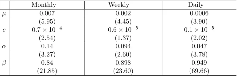
Table 2 shows the estimation results of the ARCH-NNH model with f(x) = jxj :7 For each frequency, we report estimation results of the model without any constraint on as well as with constraint of = 1. At …rst, we estimate the model without any constraint
7Notice that the coe¢cient of the lag of the squared return; ;is compatible with the asymptotic theory
because <0:58:If we assume that ("t) is iid N(0,1), then 4"= 3and we need0< < p13(= 0:577:::)in
on and all coe¢cients are tested to be signi…cant except for of the weekly frequency. The estimates of for the monthly and daily frequencies are close to unity (1:05 and 1:10
respectively) and we are not able to reject the null hypothesis of = 1. The estimation results of the model with constraint of = 1are quite similar to those of the model without constraint, and every estimate of the model without constraint is statistically signi…cant. Hence, f(x) = jxj appears to be better in describing the volatility of the stock return series, and we are going to use this function for our simulation and forecasting evaluation.
Not only is the ARCH-NNH model statistically appropriate, but the model con…rms economic thoughts. As expected, the default premium is positively related to stock return volatility, which is compatible with Schwert (1989). It is not surprising that stock market is more volatile when default risk is high.
The estimation results of GARCH(1,1) are reported in Table 3. Consistent with other empirical …ndings, the estimated + (ARCH e¤ect) is very close to unity, suggestive of the IGARCH behavior. FIGARCH 8 estimation results are given in Table 4. For each
frequency, we report both FIGARCH(1,d,1) and FIGARCH(1,d,0) estimation results. For the monthly frequency, FIGARCH(1,d,1) is preferred because estimates of d and are tested to be insigni…cant in FIGARCH(1,d,0). On the other hand, FIGARCH(1,d,0) is preferred for the weekly and daily frequencies because estimates of are insigni…cant in FIGARCH(1,d,1). Hence, we are going to use FIGARCH(1,d,1) for the monthly frequency and FIGARCH(1,d,0) for the weekly and daily frequencies in our simulation and forecasting evaluation. The long-run dynamics are modeled by the fractional di¤erencing parameterd;
and it is estimated 0:67; 0:37 and 0:30 for the selected FIGARCH model at the monthly, weekly and daily frequencies respectively. The null hypothesis of d = 0:5 is rejected in the daily case, but it is not rejected in the monthly and weekly cases. While the null hypothesis of d= 1 is clearly rejected in the weekly and daily cases, it is rejected only at 10% signi…cance level in the monthly case.
4.2 Exchange Rate Return Volatility
In their portfolio selection model of exchange rate determination, Hagiwara and Herce (1999) showed that the interest rate di¤erential between countries (absolute value or squared) is related to exchange rate return volatility. We apply this …nding to the ARCH-NNH model. Based on the model of Hagiwara and Herce (1999), we estimate the following models;
yt = b0+b1yy 1+b2yt 2+b3xt 1+ t"t;
2
t = ( t 1"t 1)2+ jxt 1j ARCH-N N H 2
t = c+ ( t 1"t 1)2+ 2t 1 GARCH(1;1)
where yt denotes the exchange rate return series in percentage form, yt = 100 (lnPt
lnPt 1)withPt=UK pound=US dollar, andxtrepresents eurocurrency interest rate spreads
8The G@RCH by Laurent and Peters is used for FIGARCH estimation and forecast. We …xed the
between US and UK(xt=rU S;t rU K;t). The mean equation forytis exactly same as that
of Hagiwara & Herce (1999). We obtained weekly observations of the exchange rate for UK pound and one-month eurocurrency interest rate for US and UK.9 The sample period is from 21 October 1983 to 31 December 2004 (1107 observations).
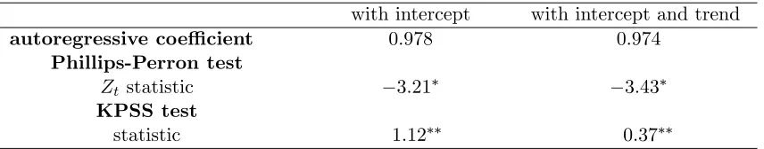
Table 5 shows that unit root tests for the interest rate di¤erential support the presence of a unit root. The estimated autoregressive coe¢cient is very close to unity in both cases. Phillips-Perron tests are unable to reject the null hypothesis of a unit root. KPSS tests reject the null hypothesis of stationarity at 1% signi…cance level.
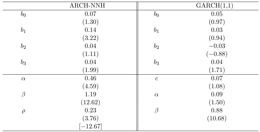
The estimation results are summarized and presented in Table 6. The estimation result of the ARCH-NNH model shows that it works well for the exchange rate return volatility. Most estimates are tested to be signi…cant and the null hypothesis of = 1is also rejected, which means a nonlinear function is clearly needed in this case. Roughly, the positivity of^b3
supports the uncovered interest parity. The absolute values of the interest rate di¤erentials are positively related to exchange rate return volatility, which is compatible with Hagiwara & Herce (1999). On the other hand, GARCH(1,1) performs very poorly and most estimates are insigni…cant.
5
Forecast Evaluation
We evaluate out-of-sample volatility forecasts of three models in the previous stock return volatility application; ARCH-NNH, GARCH(1,1), and FIGARCH(1,d,q)10. A rolling
fore-cast procedure is adapted; i.e., each forefore-cast is based on the estimated parameters from the previous (970 monthly, 979 weekly and 3688 daily) observations. We obtained 44 monthly forecasts for the November 1999 to June 2003 out-of-sample period. And, we obtained 100 weekly forecasts for the 3 August 2001 to 27 June 2003 out-of-sample period and 250 daily forecasts for the 1 July 2002 to 30 June 2003 out-of-sample period.
To evaluate the accuracy of volatility forecasts, they have to be compared with actual volatility, which cannot be observed. It is common in practice to de…ne actual volatility as squared observed returns, which for one-day ahead volatility is equal to
y2T+1 = 2T+1"2T+1:
However, the squared error term"2
T+1will vary widely and this implies that only a relatively
small part is attributable to 2T+1: An alternative approach which addresses this problem has been suggested. Refer to Andersen et al (2003) for a theoretical underpinning for the use of ‘realized volatility’. They employ the theory of quadratic variation to show that realized volatility computed from high-frequency intraperiod returns is an unbiased and e¤ectively error-free measure of return volatility.
9From the Datastream. The exchange rates are sampled on every Friday and the interest rates are
sampled on every Wednesday.
1 0Again, q = 1for the monthly frequency and q = 0for the weekly and daily frequencies following the
As a proxy for actual volatility, we use ‘realized volatility’ instead of squared returns. The measure for monthly volatility is the sum of squared daily returns:
2
t = Nt
X
i=1
(yit t)2;
where there are Nt daily returns yit in month t and t is the average of daily returns yit
in the month. It turned out that subtracting the average has only negligible e¤ect in the monthly case. Since the mean returns are smaller for higher frequencies, we assume that
= 0 for the weekly and daily frequencies. Hence, the measure for weekly volatility is the sum of squared daily returns. The daily realized volatility is de…ned as the sum of the squared overnight, close-to-open, and the cumulative squared 30-minute intraday returns.
In order to assess predictive abilities of models, we use the regression-based method and the mean absolute error (MAE). As the …rst method, we report on R2 as calculated from the OLS regression
2
T+1 =a+b^2T+1+"; (9)
where ^2T+1 denotes one-period ahead volatility forecasts. This appears to be the most commonly used method in the literature when measures for volatility are computed with ‘realized volatility’ as the sum of squared intraperiod returns. If volatility forecasts are unbiased, then a= 0 and b = 1. We test these hypotheses using the standard regression method with adjustment followed by Andrews and Monahan (1992) to account for the error covariance. The quadratic spectral kernel with automatic bandwidth selection is used to obtain heteroskedasticity and autocorrelation consistent covariance estimates.
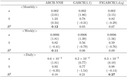
Table 7 presents forecasting performance results evaluated on the regression-based method. It shows that the ARCH-NNH model outperforms GARCH (1,1) and FIGARCH at the monthly and weekly frequencies. The null hypothesis of b= 1 is not rejected in every case. The estimates for a are very small and close to zero, but the null hypothesis of a = 0 is rejected in some cases. The comparison of forecasting ability between models is done by the R2 statistic. For the monthly frequency, R2 of the ARCH-NNH model is 0:12, which
is higher than that of GARCH(1,1), 0.05, and FIGARCH, 0.07. The weekly case shows the similar result that the ARCH-NNH model performs better than the other models. For the daily frequency, the FIGARCH model has the highest R2; 0:27: The result that R2s
in the daily case are bigger than those of other frequencies seems to be originated from the fact that the daily realized volatility is constructed by intraday returns. Comparison between GARCH(1,1) and FIGARCH shows that FIGARCH performs slightly better than GARCH(1,1) at every frequency.
We also evaluate the volatility forecasts on the basis of the mean absolute error (MAE) and test the null hypotheses of equal MAE by the Diebold and Mariano (1995) test pro-cedure. The null maintains that the predictive performance of the best performing model relative to another model is not di¤erent. First, de…ne loss di¤erential between MAEs from two forecasting models
So, the null hypothesis is E(dt) = 0:This hypothesis is evaluated using the statistic
D1 =
d q
2 ^fd(0)=N
(10)
where dis the sample mean loss di¤erential d= N1
N P t=1
dt ,f^d(0) is a consistent estimate
of the spectral density function of the loss di¤erential at frequency 0, and N is the num-ber of forecasts. To compute f^d(0), Diebold and Mariano (1995) suggest the uniform, or
rectangular, lag window with bandwidth parameter k 1 for forecast horizonk. Since we deal with only one-step ahead forecasts, we have2 ^fd(0) = N1
N P t=1
dt d 2:Under the null
hypothesis,D1 N(0;1)asymptotically.
However, since N is relatively small for the monthly case (N = 44), we add another statistic D2 for the exact …nite-sample test of the monthly case, which is also developed
by Diebold and Mariano (1995). The null hypothesis is a zero median loss di¤erential,
med(dt) = 0, and this hypothesis is evaluated using the statistic
D2 =
N X
t=1
I+(dt) (11)
where
I+(dt) = 1 if dt>0
= 0 otherwise.
Signi…cance is assessed using a table of the cumulative binomial distribution with parameters
N and 12 under the null hypothesis.
Forecasting evaluation based on MAE is reported in Table 8. The lowest MAEs come from GARCH(1,1) for the monthly frequency, from the ARCH-NNH model for the weekly frequency, and from FIGARCH for the daily frequency. It is hard to select the best per-forming model from the evaluation result based on MAE even after we consider the fore-cast accuracy test. The forefore-cast accuracy tests using D1 and D2 show the same result
in the monthly case. For the monthly frequency, the forecast accuracy tests show that GARCH(1,1) performs signi…cantly better than the ARCH-NNH model, but its perfor-mance is not signi…cantly di¤erent from that of FIGARCH. For the weekly frequency, the ARCH-NNH model has the lowest MAE, but there is no signi…cant di¤erence in forecasting ability between models according to the forecast accuracy test. At the daily frequency, the forecast of the FIGARCH model is signi…cantly better than that of GARCH(1,1), but it is not signi…cantly di¤erent from that of the ARCH-NNH model.
6
Concluding Remarks
As explained in the introduction, econometricians have been using ARCH type models with persistent covariates to model the volatility of economic and …nancial time series. While the e¤ect of persistent covariates on various characteristics of volatility has been ignored, this paper …lls this gap and gives theoretic understandings about ARCH models with persistent covariates. We provide the asymptotic theories showing how persistent covariates in ARCH models would a¤ect various characteristics of volatility.
There are two more stylized facts about volatility in …nancial time series which we did not consider in this paper. One is the leverage e¤ect in stock return series, and the ARCH-NNH model can easily deal with the issue in the same way as Glostenet al (1993) used a dummy variable. The other is the co-movement in volatility. If we look at exchange rate returns for di¤erent currencies, we observe big movements in one currency being matched by big movements in another. This suggests the importance of multivariate models in modelling cross-correlations in di¤erent markets. Multivariate or panel models using ARCH-NNH processes could provide a proper way to explain volatility spillover in foreign exchange markets. This task awaits further research.
The forecast evaluation in this paper shows that the ARCH-NNH model outperforms other standard models at relatively lower frequencies. Hence, if we apply an ARCH-NNH model in a price determination model, it could produce better forecasts of a price level such as the exchange rate or stock return. One of the important issues in …nance is whether stock returns are predictable by macroeconomic variables. Much of the literature pertaining to this issue uses a linear function in mean equation of stock return. Nonlinear functions of persistent macroeconomic variables can be used to investigate both the mean and volatility equations of asset price returns. These possibilities will be addressed in future research.
References
Andersen, T.G., Bollerslev, T., Diebold, F.X. and Labys, P. (2003), "Modeling and fore-casting realized volatility,"Econometrica,71, 529-626.
Andrews, D.W.K. and Monahan, J. (1992), "An improved heteroskedasticity and autocor-relation consistent covariance matrix estimator,"Econometrica,60, 953-966.
Baillie, R.T., Bollerslev, T., and Mikkelsen, H.O. (1996), "Fractionally integrated general-ized autoregressive conditional heteroskedasticity,"Journal of Econometrics,74, 3-30.
Bartlett, M.S. (1946), "On the theoretical speci…cation of sampling properties of autocor-related time series,"Journal of the Royal Statistical Society, B 8, 24-41.
Bollerslev, T. (1986), "Generalized autoregressive conditional heteroskedasticity," Journal of Econometrics, 31, 307-327.
Bollerslev, T., Engle, R.F., and Nelson, D.B. (1994): "ARCH models," In R.F. Engle and D.L. McFadden, eds., Handbook of Econometrics, Vol. 4, 2959-3038, Elsevier: Amsterdam.
Bollerslev, T. and Wooldridge, J.M. (1992), "Quasi-maximum likelihood estimation and inference in dynamic models with time-varying covariances,"Econometric reviews,11, 143-172.
Chung, H. and Park, J.Y. (2004), "Nonstationary nonlinear heteroskedasticity in regres-sion," mimeograph, Department of Economics, Rice University.
Ding, Z. and Granger, C.W.J. (1996), "Modeling volatility persistence of speculative returns: A new approach," Journal of Econometrics,73, 185-215.
Ding, Z., Granger, C.W.J., and Engle, R.F. (1993), "A long memory property of stock market returns and a new model,"Journal of Empirical Finance, 1, 83-106.
Diebold, F.X. and Mariano, R.S. (1995), "Comparing predictive accuracy,"Journal of Busi-ness and Economic Statistics,13, 253-263.
Diebold, F.X. and Inoue, A. (2001), "Long memory and regime switching," Journal of Econometrics, 105, 131-159.
Engle, R.F. (1982), "Autoregressive conditional heteroskedasticity with estimates of the variance of U.K. In‡ation," Econometrica, 50, 987-1008.
Engle, R.F. and Lee, G.J. (1999), A long-run and short-run component model of stock return volatility, in Engle R. and H. White ed. Cointegration, Causality, and Forecasting: A Festschrift in Honour of Clive W.J. Granger, Chapter 10, 475-497, Oxford University Press.
Engle, R.F. and Patton, A.J. (2001), "What good is a volatility model?," Quantitative Finance, 1(2), 237-245.
Glosten, L.R., Jagannathan, R. and Runkle, D. (1993), "On the relation between the ex-pected value and the volatility of nominal excess returns on stocks," Journal of Finance, 48, 1779-1801.
Granger, C.W.J. and Hyung, N. (2004), "Occasional structural breaks and long memory with an application to the S&P 500 absolute stock returns,"Journal of Empirical Finance, 11, 399-421.
He, C. and Teräsvirta, T. (1999), "Properties of moments of a family of GARCH processes," Journal of Econometrics,92, 173-192.
Hagiwara, M. and Herce, M.A. (1999), "Endogenous exchange rate volatility, trading volume and interest rate di¤erentials in a model of portfolio selection," Review of International Economics, 7(2), 202-218.
Han, H. and Park, J.Y. (2006), "ARCH models with persistent covariates: asymptotic distri-bution theory of QMLE and IGARCH behavior," mimeograph, Department of Economics, National University of Singapore.
Hillebrand, E. (2005), "Neglecting parameter changes in GARCH models," Journal of Econometrics, 129, 121-138.
Hodrick R.J. (1989), "Risk, uncertainty, and exchange rates," Journal of Monetary Eco-nomics, 23, 433-459.
Hol, E.M.J.H. (2003), Empirical studies on volatility in international stock markets. Dor-drecht: Kluwer Academic.
Hyung, N., Poon, S.H. and Granger, C.W.J. (2006), "A source of long memory in volatility," mimeograph, Manchester Business School, University of Manchester.
Kwiatkowski, D., Phillips, P.C.B., Schmidt, P. and Shin, Y. (1992), "Testing the null hy-pothesis of stationarity against the alternative of a unit root,"Journal of Econometrics, 54, 159-178.
Lamoureux, C.G. and Lastrapes, W.D. (1990), "Heteroskedasticity in stock return data: volume versus GARCH e¤ects,"Journal of Finance, 45, 221-229.
Laurent, S. and Peters, J.P. (2005), "G@RCH 4.0, Estimating and forecasting ARCH mod-els," Timberlake Consultants.
Lee, S.W. and Hansen, B.E. (1994), "Asymptotic theory for the GARCH(1,1) quasi-maximum likelihood estimator,"Econometric Theory, 10, 29-52.
Lumsdaine, R.L. (1996), "Consistency and asymptotic normality of the quasi-maximum like-lihood estimator in IGARCH(1,1) and covariance stationary GARCH(1,1) models," Econo-metrica, 64, 575-596.
Mikosch, T. and Starica, C. (2004), "Nonstationarities in …nancial time series, the long-range dependence, and the IGARCH e¤ects," The Review of Economics and Statistics,86, 378-390.
Nelson, D.B. (1990), "Stationarity and persistence in the GARCH(1,1,) model," Economet-ric Theory, 6, 318-334.
Park, J.Y. (2002), "Nonstationary nonlinear heteroskedasticity,"Journal of Econometrics, 110, 383-415.
Park, J.Y. (2003), "Weak unit root," mimeograph, Department of Economics, Rice Univer-sity.
Park, J.Y. and Phillips, P.C.B. (1999), "Asymptotics for nonlinear transformations of inte-grated time series," Econometric Theory, 15, 269-298.
Park, J.Y. and Phillips, P.C.B. (2001), "Nonlinear regressions with integrated time series," Econometrica, 69, 117-161.
Phillips, P.C.B. (1987), "Towards a uni…ed asymptotic theory for autoregression," Bio-metrika, 74, 535-547.
Phillips, P.C.B. and Perron, P. (1988), "Testing for a unit root in time series regression," Biometrika, 75, 335-346.
Poon, S.H. and Granger, C.W.J. (2003), "Forecasting volatility in …nancial markets," Jour-nal of Economic Literature,41, 478-539.
Robinson, P.M. and Za¤aroni, P. (2005), "Pseudo-maximum likelihood estimation of ARCH(1) models," Annals of Statistics, forthcoming.
Schwert, G.W. (1989), "Why does stock market volatility change over time?," Journal of Finance, 44, 1115-1154.
Stock, J.H. (1994): "Unit roots and structural breaks," In R.F. Engle and D.L. McFadden, eds.,Handbook of Econometrics, Vol. 4, 2739-2841, Elsevier: Amsterdam.
Appendix A. Useful lemmas and their proofs
The proofs of the theorems in the paper rely on the results from the following lemmas. For the lemmas and their proofs, we let Assumptions 1 and 2 hold.
Lemma 1 Let T be a transformation on R. De…ne
M1n= n X
t=1
T(xt) and M2n= n X
t=1
T2(xt):
(a) If T 2I; we have under Assumption 4S(b)
n 1=2M1n!dLc(1;0) Z 1
1
T(x)dx
n 1=2M2n!dLc(1;0) Z 1
1
T2(x)dx
as n! 1:
(b) If T 2 H with asymptotic order and limit homogeneous function f and if we let
n= (pn); we have under Assumption 4W(b)
(n n) 1M1n!d Z 1
0
f(Vc(r))dr
(n 2n) 1M2n!d Z 1
0
f2(Vc(r))dr
as n! 1:
The weak convergences in (a) and (b) hold jointly.
Proof of Lemma 1. See Park (2002, 2003). The classes of I and H transformations are closed under the product operation. If T 2 I, then T2 2 I. And if T 2 H with limit homogeneous functionf, thenT22Hwith limit homogeneous functionf2:IfT22I, then
n 1=2M2n=pn Z 1
0
T2(pnVcn(r))dr:
IfT2 2Hwith limit homogeneous function f2 and asymptotic order 2n;then
(n 2n) 1M2n=
1
n n X
t=1
T2(xt)
2
n
1
n n X
t=1
f2(p1
nxt):
Lemma 2Let T be a transformation on R,and let utbe a martingale di¤erence sequence
(MDS) with respect toFtsuch that E(ut2jFt 1) = 2ua.s. for eachtandsuptE(jutj2+ jFt 1)<
1 a.s. for some >0:De…ne
U1n= n X
t=1
T(xt)ut and U2n= n X
t=1
(a) If T 2I; then U1n, U2n=Op(n1=4) respectively under Assumption 4S and 5S.
(b) If T 2 H with asymptotic order ; and if we let n = (pn); then U1n =Op(n1=2 n)
and U2n=Op(n1=2 2n) respectively under Assumption 4W and 5W.
Proof of Lemma 2. See Park (2003).
For example, let us consider asymptotic limits of Pn
t=1
T(xt)"2t and n P t=1
T(xt)"4t: Notice
that"2
t 1 and "4t 4" are MDSs. If T 2I, then
1 p n n X t=1
T(xt)"2t =
1 p n n X t=1
T(xt) +
1 p n n X t=1
T(xt) "2t 1
= p1
n n X
t=1
T(xt) +p1
nOp(n
1=4)
!dLc(1;0)
Z 1
1
T(x)dx
and 1 p n n X t=1
T(xt)"4t = p1
n n X
t=1
T(xt) 4"+p1
n n X
t=1
T(xt) "4t 4"
= 4"p1
n n X
t=1
T(xt) +
1
p
nOp(n
1=4)
!d 4"Lc(1;0) Z 1
1
T(x)dx:
Lemma 3 Let T be a transformation on Rand denote pk the density of (vkt) with respect
to measure m on R. De…ne
Bn= n X
t=k+1
T(xt)T(xt k):
(a) If T 2I; we have under Assumption 3S
n 1=2Bn!dLc(1;0) Z 1
1 k
T(x)dx
as n! 1;where k=R1
1T(x+y)pk(y)m(dy):
(b) If T 2 H with asymptotic order and limit homogeneous function f and if we let
n= (pn); we have under Assumption 3W
(n 2n) 1Bn!d Z 1
0
f2(Vc(r))dr
Proof of Lemma 3.
xt = 1 c
n k
xt k+ k 1
X
i=0
1 c
n i
vt i
= xt k+ k 1
X
i=0
vt i+q1(
c
n; xt k) +q2 c
n; vt 1; vt 2; :::; vt k+1
where
q1(
c
n; xt k) = 1 c n
k
1 xt k
and
q2 c
n; vt 1; vt 2; :::; vt k+1 = k 1
X
i=1
1 c
n i
1 vt i:
Letvkt= kP1
i=0
vt i. Notice thatq1; q2 !0as n! 1:We have
n X
t=k+1
T(xt)T(xt k) = n X
t=k+1
T(xt k+vkt+q1+q2)T(xt k)
=
n X
t=k+1
T(xt k+vkt)T(xt k) + n X
t=k+1
DnT(xt k)
whereDn=T(xt k+vkt+q1+q2) T(xt k+vkt):
IfT 2I, thenDn2I andDnT 2I. SincejDnT(x)j jD1T(x)jfor allx2R, we apply
Lebesgue’s Dominated Convergence Theorem and, slightly abusing notation, obtain
n 1=2 n X
t=k+1
DnT(xt k) !d lim
n!1Lc(1;0)
Z 1
1
DnT(x)dx
= Lc(1;0) Z 1
1
lim
n!1DnT(x)dx= 0:
Thus, we have
n 1=2 n X
t=k+1
T(xt)T(xt k)
= n 1=2 n X
t=k+1
T(xt k+vkt)T(xt k) +op(1)
!d Lc(1;0)
Z 1
1
kT(x)dx:
IfT 2H, then we haveDn2Hwhere its asymptotic order is and its limit homogeneous
function is zero. Hence, we have DnT(x)2Hwhere its asymptotic order is and its limit
homogeneous function is zero. Thus, we have
(n n) 1 n X
t=k+1
DnT(xt k)!p0:
Therefore,
(n 2n) 1
n X
t=k+1
T(xt)T(xt k)
= (n 2n) 1
n X
t=k+1
T(xt k+vkt)T(xt k) +op(1)
!d
Z 1
0
f2(Vc(r))dr:
See the proof of Theorem 1 of Park (2002) for the third line.
Lemma 4Suppose that 0< <1andvn! 1monotonically asn! 1:If v1n n P
k=1
f(xt)!d Q; then, as n! 1;
1 vn n 1 X k=0 k n k X t=1
f(xt)!d
1 1 Q:
Proof of Lemma 4. LetCn= v1
n
n P k=1
f(xt) Q:ThenCn!d0and n P k=1
f(xt) =vn(Q+Cn):
1 vn n 1 X k=0 k n kX
t=1
f(xt) =
1
vn n 1
X
k=0
k[v
n kQ+vn kCn k]
= Q 1 vn
S+ 1
vn T
whereS =nP1
k=0
kv
n k andT = nP1
k=0
kv
n kCn k:
At …rst, we are going to show that v1
nS!0:Since
S S= vn+ n 2
X
i=0
1+i(v
n i vn 1 i) + nv1;
we have
1
vnS =
1 1 + 1 vn 1 1
"n 2 X
i=0
1+i(v
n i vn 1 i) + nv1
#
! 1
The last line follows because
1
vn "n 2
X
i=0
1+i(v
n i vn 1 i) + nv1
#
1
vnV +
2+:::+ n = 1 vnV
(1 n)
1 !0
whereV = max
t (vt vt 1; v1) for2 t n:
Now, We need to show that v1
nT !p 0: Recall that!d and !p are identical when the
convergence is to a nonrandom limit. Therefore, Cn !d 0 implies Cn !p 0: The stated
result follows because
1 vn T n 1 X k=0
kvn k vn j
Cn kj
< n 1
X
k=0
k
jCn kj !p0:
Here, the convergence to zero follows becauseCn!p 0 and0< <1. This completes the
proof.
Appendix B. Proofs of the main results
Proof of Theorem 1. Suppose thatvn =pn forf 2 I and vn =n 2(pn) forf 2 H.
At …rst, we need to obtain asymptotic limits for the following three sample moments:
X
y2t; Xyt4; Xyt2yt k2 :
The …rst sample moment is
n X
t=1
y2t =
n X
t=1 2
t"2t = n X
t=1
f(xt) + y2t 1 "2t
= n X t=1 n 1 X j=0
jf(xt j) Qj h=0
"2t h
= n 1 X j=0 j n X t=1
f(xt j) + n 1 X j=0 j n X t=1
f(xt j) j Q h=0
"2t h 1
!
Since
j Q
h=0
"2t h 1
!
forj= 0;1; :::; n 1 are MDSs,
1 vn n 1 X j=0 j n X t=1
f(xt j) j Q
h=0
"2t h 1
!
by lemma 2 and Lemma 4. Therefore, 1 p n n X t=1
yt2 = p1
n n 1 X j=0 j n X t=1
f(xt j) +op(1)
= p1
n n 1 X j=0 j n j X t=1
f(xt) +op(1):
Applying Lemmas 1 and 4 gives us
1 p n n X t=1
yt2 !d
1
1 Lc(1;0)
Z 1
1
f(s)ds.
Similarly, for f 2H, we have
(pn) 1
n n X
t=1
y2t = (
pn) 1
n n 1 X j=0 j n j X t=1
f(xt) +op(1)
!d
1 1
Z 1
0
f(Vc(r))dr:
The second sample moment is
n X
t=1
y4t =
n X
t=1
f(xt)2"4t + 2 n X
t=1
f(xt)yt2 1"4t+ 2 n X
t=1
yt4 1"4t
=
n X
t=1
f(xt)2"4t + 2
n 1 X i=1 i n X
t=1+i
f(xt)f(xt i)"4t i Q
h=1
"2t h
+ 2
n X
t=2
yt4 1"4t
= " 4 " n X t=1
f(xt)2+ 2 4" n 1 X i=1 i n X
t=1+i
f(xt)f(xt i) #
+ 2
n X
t=2
yt4 1"4t
+ 2 6 6 4 n P t=1
f(xt)2("4t 4")
+2nP1
i=1
i Pn t=1+i
f(xt)f(xt i) "4t i Q
h=1
"2
t h 4" 3
7 7 5:
Since "4
t i Q
h=1
"2
t h 4" are MDSs, similarly as the equation (A1), we have
1
vn " n
X
t=1
f(xt)2("4t 4") + 2 n 1 X i=1 i n X
t=1+i
f(xt)f(xt i) "4t i Q
h=1
"2t h 4" #