The Chinese Chaos Game

Munich Personal RePEc Archive

The Chinese Chaos Game

Raul, Matsushita and Iram, Gleria and Annibal, Figueiredo

and Sergio, Da Silva

Federal University of Santa Catarina

2006

The Chinese Chaos Game

Raul Matsushita

,

Iram Gleria

,

Annibal Figueiredo

,

Sergio Da Silva

a

Department of Statistics, University of Brasilia, 70910900 Brasilia DF, Brazil

b

Department of Physics, Federal University of Alagoas, 57072970 Maceio AL, Brazil

c

Department of Physics, University of Brasilia, 70910900 Brasilia DF, Brazil

d

Department of Economics, Federal University of Santa Catarina, 88049970 Florianopolis SC, Brazil

Abstract

The yuan-dollar returns prior to the 2005 revaluation show a Sierpinski triangle in an iterated function system clumpiness test. Yet the fractal vanishes after the revaluation. The Sierpinski commonly emerges in the chaos game, where randomness coexists with deterministic rules [2, 3]. Here it is explained by the yuan’s pegs to the US dollar, which made more than half of the data points close to zero. Extra data from the Brazilian and Argentine experiences do confirm that the fractal emerges whenever exchange rate pegs are kept for too long.

PACS: 05.40.+j; 02.50.-r

Keywords: Chaos game; iterated function systems; yuan-dollar exchange rate; Chinese monetary policy; exchange rate pegs

1. Introduction

China introduced market reforms in the early 1980s. Only a third of the economy is now directly state-controlled. The country has become a global economic force and joined the World Trade Organization in 2001. It currently exports more information technology goods than the United States. It also created a commodity-market boom, and turned into the world’s third largest car market. Over a dozen Chinese companies are on the Fortune 500 list.

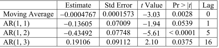
From 16 June 1994 to 21 July 2005 China pegged its currency, the yuan, at 8.28 to the dollar. Following the 2005 revaluation the yuan’s central rate against the dollar was shifted by 2.1 percent, to 8.11. From then on, the yuan is said to be linked to a basket of currencies, the central parities of which are set at the end of each day. The Chinese central bank called it a “managed floating exchange-rate regime”. Yet as of 30 March 2006, the yuan has risen by a mere one percent against the dollar (left-hand chart in Figure 1). Zhou Xiaochuan, the central bank’s governor, said that he understood it was in China’s interest to make the yuan more flexible over time, but that this needed to be gradual.

US political pressure on the yuan is mounting, as a result. Yet it seems reasonable for the Chinese government not to allow the yuan rise much against the dollar while the dollar itself remains climbing. The yuan has risen against the euro, and

∗

Corresponding author.

2

its trade-weighted value rose in 2005 (Figure 1). And the trade-weighted rate has a much greater effect on both China’s economy and the world’s.

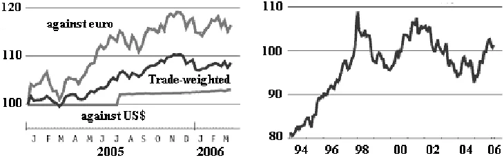
The yuan’s revaluation of 2005 was not the first big episode of foreign exchange intervention (Figure 2). However, the last revaluation brought a fundamental change. Prior to the revaluation, a mix of intervention and random shocks hitting China’s trade balance generated a fractal pattern in the yuan-dollar rate series [1]. The fractal, a Sierpinski triangle, is indicative that the Chinese central bank was playing the “chaos game” [2, 3]. The fractal vanishes from 22 July 2005 on (Figure 8), though some pattern can still be detected.

Section 2 details the concepts above and presents analysis. Section 3 explains the origin of the yuan’s fractal structure. And Section 4 concludes.

2. Analysis

Daily data from the yuan-dollar rate were taken from the Federal Reserve website. It ranges from 2 January 1981 to 31 March 2006. Figure 2 displays the time evolution of rate Zt together with single returns Xt = Zt – Zt–1. We consider X_t =0 whenever

0001 . 0 |

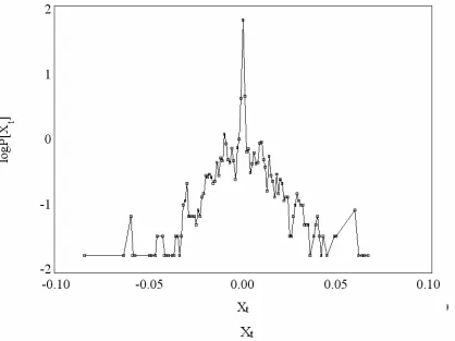
|Z_t −Z_t−1 ≤ . The spikes correspond to the biggest episodes of foreign exchange intervention (Xt > 0.05). Figure 3 shows the probability density function in logs with

the days of intervention dropped. A stationary ARMA seems inadequate to model data. Indeed there is marked asymmetry and a peak higher than that of a Gaussian distribution. (Figure 4 shows pieces of the entire series.)

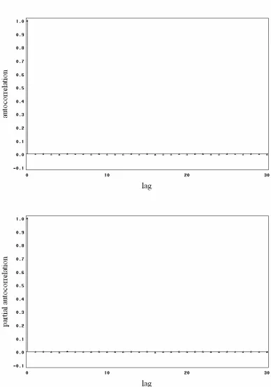
Figure 5 shows the autocorrelation and partial autocorrelation functions for Xt.

The autocorrelations are not significantly different from zero after the first lag. Thus we cannot dismiss Xt as an uncorrelated random process. We carried out other statistical

tests and they also failed to detect autocorrelation (Table 1). Because distinguishing an IID process from a non-IID is not possible on the basis of second order properties, we also considered higher order ones and took squared single returns. But all these failed to detect autocorrelation. However, autocorrelation is clear-cut for portions of data (Figure 6).

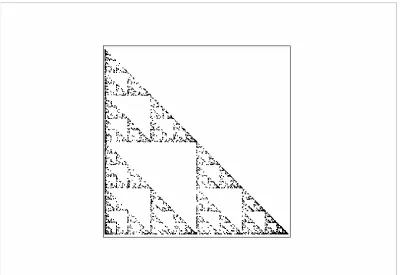
Then we performed an iterated function system (IFS) clumpiness test using SAS

(and also Chaos Data Analyzer [4]). Here while white noise fills a screen uniformly, correlated noise generates localized clumps. And, indeed, the data idiosyncratically clump together and form a Sierpinski triangle (upper chart in Figure 7). More than half, 64 percent to be precise, of the data points near zero. This is due to exchange rate pegs. Also, 16 percent are positive values, and 20 percent are negative values. Commonly the Sierpinski stems from a deterministic rule implemented in a random fashion. This is the chaos game [2, 3, 5]. Here the deterministic rules can be thought of as the central bank interventionist behavior over the pegs, while defending the yuan against random shocks. Figure 8 shows the IFSs for portions of data. The fractal vanishes after the 2005 revaluation.

The IFS, the chaos game representation, and the results above are now explained in more detail (this borrows in part from [6]). An iterated function system is a set of functions f_i:ℜ → ℜ2 2 where f_i( )θ =M(θ θ− _i)+θ_i, 1≤ ≤i n, θ is any point ( , )r s ,

( , ) i r s

θ is a given fixed point on the plane associated with each particular f_i, and

(0,1)

M∈ is a multiplier.

Thus each function f_i is a linear contraction of the plane. If we take

( ) ( ) ( ) ( )

i i i i i

( , )r s

θ , then the distance between the arbitrary point θ and the fixed point θ_i will

decrease by a factor of M. SinceM∈(0,1), the arbitrary point θ will approach the fixed point θ_i. So multiplier M is called the contraction factor of the function.

For any point ( , )θ r s , if one iterates the function f_i, the result will converge to

the fixed point ( , )θ r s_{i i} regardless of the value of M∈(0,1). The sequence of points in

the plane obtained as the result of iterating each of the f_i functions of a given point

0 0

( ,r s )

θ is called the orbit of θ( ,r s_{0 0}). The fixed point is called the seed.

A simple graphical technique using the IFS is the chaos game algorithm [2],

which aims to map a sequence of numbers into a subset of ℜ2_{. The chaos game}

algorithm thus produces a visual representation of the sequence of random numbers. The technique is intended as a visual aid to more conventional statistically-oriented methods to find non-randomness within pseudo random data sets.

The chaos game algorithm uses the IFS with particular constraints, namely (1) a probability πi is associated with each function fi; (2) M = ½, which means that the

midpoint of a current point and the fixed point ( , )r si i is taken when evaluating ( )f θ ; (3) introduction of a mechanism for generating a sequence of random numbers in the interval (0,1) which corresponds to the probabilities π_i given in the IFS table; and (4)

choice of a seed point ( ,r s_{0 0})∈ℜ2. An additional implementation is to choose the number of vertices to be used, since each equation f_i is generally associated with a vertex of a geometric figure. Four vertices are usually taken because this can be easily mapped to the corners of a computer display. The resulting image is referred to as the chaos game representation.

To apply (or “play”) the chaos game algorithm given a seed point ( ,r s_{0 0}) is to use a random number to select the jth equation, f_j. The point f r s_j( ,_{0 0}) is plotted. With the next play, f_k(f r s_j( ,_{0 0})) is plotted, then f f_i( _k(f r s_j( ,_{0 0}))), and so on. This process is iterated for some large number of steps. The orbit that is created will, with a probability of 1, tend toward the same orbit for any initial seed point in ℜ2.

If the numbers are random, then the figure generated will tend toward the orbit. If the numbers are not random, or there exists correlation in data, then one may find features in the visual representation of the sequence corresponding to these anomalies.

Suppose that the chaos game is played with a randomly generated time series

n t t

W}_{1 3}

{ _≤≤ . Then sort this sequence as W₍₁₎ ≤W₍₂₎ ≤"≤W_{(3 )n} , where each W_(k) is the kth

order statistic from {W_t}_1≤t≤3n. Now divide the sequence equally into three parts

n t t

W₍₎}_1≤≤

{ , {W_(t)}_n<t≤2n, and {W_(t)}_2n<t≤3n. One can thus define the IFS as follows. Step 1: choose a seed point ( ,r s_{0 0})∈ℜ2. Step 2: for t = 1 to 3n,

if W_t∈{W_(t)}_1≤t≤n then make r_t =0.5(r_t−1+1) and s_t =0.5(s_t−1+1); if W_t∈{W_(t)}_n≤t≤2n then make r_t =0.5(r_t−1+0) and s_t =0.5(s_t−1+1); and if W_t∈{W_(t)}_2n≤t≤3n then make r_t =0.5(r_t−1+0) and s_t =0.5(s_t−1+0). Step 3: stop. The output will be a Sierpinski triangle similar to that in Figure 7.

However, if {W_t}_1≤t≤4n is sorted and divided into four equal parts {W_(t)}_1≤t≤n,

n t n t

W₍₎} ₂

{ _<≤ , {W_(t)}_2n<t≤3n, {W_(t)}_3n<t≤4n, and the line

4

is added to the routine in step 2, the output will be data points uniformly dense in the screen, such as those in Figure 14. Interestingly, our results for the yuan-dollar returns show a situation where the Sierpinski triangle emerges in the latter case. That happens because one out of the four rules (defined to move a point) is inactive. Put it differently, there is a dimension reduction of the game. As if one rolls a four-sided dice and one of the sides almost never come up.

The first quartile χ₁, the median χ₂, and the third quartile χ₃ are values satisfying (1) P X( _t ≤χ₁)≥0.25 and P X( _t ≥χ₁)≥0.75; (2) P X( _t ≤χ₂)≥0.50 and

2

( _t ) 0.50

P X ≥χ ≥ ; and (3) P X( _t ≤χ₃)≥0.75 and P X( _t ≥χ₃)≥0.25 (e.g. [9]). If 64 percent of the data points are null (as in the Chinese pegs), then χ₁ = χ₂ = χ₃ = 0 satisfies these three conditions. In such a situation the dimension of the chaos game is reduced.

Figures 9 and 10 present scatterplots of Xt against Xt–1. These suggest a

nonlinear deterministic structure given by X_t =J_t−1X_t−1, where J_t−1 is a deterministic input with states varying from –5 to +5 by fixed amount 0.25. It is assumed that

1 0

t

J₋ = whenever either X_t−1 =0 or X_t =0. The J can be thought of as representing episodes of central bank intervention. We find this model to be valid for 70 percent of the dataset; and state J_t−1 =0 alone represents 64 percent of data. Figure 11 shows that episodes of intervention are more frequent from 16 June 1994 on (apart from the interventions 0J_t−1 = and J_t−1 =±1). And state J_t−1 =±1 dominates from 16 June 1994 to 14 December 2004. This is not so surprising because 16 June 1994 is the date of launching of the 11-year-old peg. Interventions are also less frequent after the 2005 revaluation.

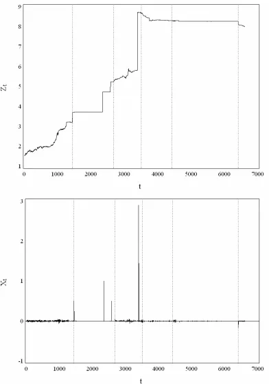
The IFS tests (Figure 8) cannot track single episodes of intervention. This is because the IFS cannot distinguish deterministic zeros from random zeros. To illustrate this, consider a model with nonadditive noise [1] given by X_t = A_t−1X_t−1, where A_t−1 is an intrinsic random variable with conditional distribution

(

)

−1 1 1 2

) 1 ( 2 1 1 0 | a p X a A

P _{t t} if a > 0,

(

)

< _{−1 2 2}

) 1 ( 2 1 0 | a p X a A

P _{t t} if a < 0, and

(

)

P _t− = _t− ≠ = ,

where 1p₁+ p₂ + p₃ = , and 0< p p p₁, ₂, ₃<1. Moreover

(

)

1 _α β

x q

X x X

P _{t t} if x > 0,

(

)

1 _α β

x q

X x X

P _{t t} if x < 0, and

(

)

P _t = _t− = = ,

where 1q₁ +q₂ +q₃ = , 0<q q q₁, ₂, ₃<1, and α,β >0 are the distribution parameters. Figure 12 shows 6,000 realizations of this model calibrated with probabilities p₁

= p₂ = 0.36, q₃ = 0.74, q₁ = q₂ = 0.115, and q₃ = 0.77, and with parameters

5 . 3

2 1 =α =

α , and β₁ =β₂ =747. The model replicates part of the yuan behavior [1]

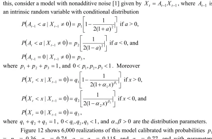
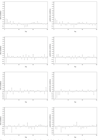
We can also focus on the period after the 2005 revaluation. Thanks to the fewer observations, we discard the use of a GARCH model. Yet the autocorrelations (Figure 6) (significant at lags 5, 15, and 16) suggest a cyclical pattern each trading week. This subset of data can then be modeled by an adjusted autoregressive model such as

1 5 16

0.0005 0.14 0.43 0.19

t t t t t

X = − − X₋ − X ₋ + X₋ +a , where a_t is white noise with zero

mean and estimated variance 8.3 10× −6. Coefficients’ P values fall short of 5.5 percent. And the model presents the smaller value in Schwarz criterion (Table 2). As a result, mean returns can be predicted using returns of 1, 5, and 16 previous days. Obviously the model is useful as a trend-tracker only, since its explanation coefficient is too low (0.22). Despite that, it can still account for more than 1/5 of the total variation of returns.

3. Explaining the origin of the yuan’s fractal structure

The Sierpinski triangle in data prior to the last revaluation seems to originate from the yuan’s exchange rate pegs. These made more than half of the returns’ data points close to zero. To evaluate the hypothesis that it is the amount of zeros in data that causes the fractal structure, we shuffled the yuan-dollar returns dataset only to have the Sierpinski appearing again (not shown). Generally, taking pseudo-random numbers (Figure 13) with more than 50 percent of zeros (χ₁=χ₂ =χ₃ =0) suffices to generate the fractal in an IFS clumpiness test.

This can also be confirmed by extra actual data. We take these from Brazil and Argentina because these countries also experienced exchange rate pegs recently. (Data are from the Fed and Oanda websites respectively). Data from the Brazilian real–US

dollar returns during the “exchange rate anchor” over the period 3 January 1995−12

January 1999 present 11.4 percent of zeros, 58.2 percent of positive values, and 30.4 percent of negative values (χ₁= −0.0002,χ₂ =0.0002,χ₃ =0.0009). This peg of the exchange rate was not enough to produce the fractal in an IFS test (Figure 14).

Yet the Sierpinski also emerges for the Argentine peso during the “currency

board” (1991−2002). Data from 29 April 1998 to 31 December 2002 show 76.7 percent

of zeros, 12 percent of positive values, and 11.3 percent of negative values (χ₁=χ₂ =χ₃ =0). The peg was enough to produce the chaos game (Figure 15).

Finally we say a few words about the underlying dynamics of our findings. Let

t

Y be the yuan-dollar returns’ time series with the episodes of intervention dropped.

The interventions J_t are seen as dichotomous, i.e. J_t =0 if an intervention occurs at

time t, and J_t =1 in the absence of intervention. Then define a new series of returns as

a mixture of two time series given by X_t =Y J_{t t}. The Sierpinski triangle emerges from

the IFS as the probability of state J_t =0 increases. Actually the yuan-dollar returns

present more than two states J_t (Figure 11). But state J_t =0 is dominant, and this is reflected in the IFS. The same is true as for the Argentine peso-dollar returns, but this is not so for the Brazilian real-dollar returns.

4. Conclusion

6

The fractal pattern vanishes after the 2005 revaluation, though behavior does not become purely random. An adjusted autoregressive model of the period can account for more than 1/5 of the total variation of returns.

The Sierpinski in data can be explained by the yuan’s exchange rate pegs, which made more than half of the observations close to zero. Shuffling the yuan-dollar returns data still produces the Sierpinski. Generally, a pseudo-random series with more than 50 percent of zeros generates the fractal. And data from the Brazilian and Argentine experiences of exchange rate pegs do confirm that the Sierpinski originates from the amount of zeros in the time series.

Test Null Hypothesis H0 Alternative Hypothesis HA

Statistic of Test P-Value Decision

Ljung-Box Type1 White Noise No White Noise 4.67 with 120

Degrees of Freedom

~1.000

Durbin-Watson2 ρ(h) = 0

where ρ(h) is Correlation Between X(t)

and X(t + h)

ρ(h) ≠ 0 About 2.00 for h

= 1, 2, 3,..., 200. > 0.5000

McLeod–Li3 Data Set is an

IID Gaussian Sequence

Data Set is not an IID Gaussian

Sequence

0.07 with 50 Degrees of

Freedom

~1.000

Turning Points3 501 ~1.000

Difference–Sign3 405 ~1.000

Rank Test3

Data Set is an IID Sequence

Data Set is not an IID Sequence

489.248 ~0.9965 One Cannot

Reject H0

Table 1. Autocorrelation tests for the presence of white noise.

Notes

1 SAS/ETS/PROC ARIMA Version 8.2 2 SAS/ETS/PROC AUTOREG Version 8.2 3 ITSM96, Program PEST [8]

Estimate Std Error t Value Pr > |t| Lag

Moving Average −0.0004767 0.0001573 −3.03 0.0028 0

AR(1, 1) −0.13605 0.07009 −1.94 0.0539 1

AR(1, 2) −0.43492 0.07748 −5.61 < 0.0001 5

AR(1, 3) 0.19106 0.09112 2.10 0.0375 16

Table 2. Schwarz criterion for model selection for the subset of data after the 2005 revaluation.

8

Source: Thomson Datastream, J. P. Morgan Chase, The Economist

10

12

Figure 6. Autocorrelation functions (left-hand charts) and partial autocorrelation functions (right-hand charts) for subsets of data. Periods 9 April 1991–31 May 1994, 1

June 1994–30 November 1997, 1 December 1997–21 July 2005, and 22 July 2005−31

Figure 8. IFS clumpiness tests for subsets of data. From left to right, periods 2 January

1981−3 July 1986, 7 July 1986–8 April 1991, 9 April 1991–31 May 1994, 1 June 1994–

30 November 1997, 1 December 1997–21 July 2005, and 22 July 2005−31 March 2006.

16

Figure 9. Scatterplot for the entire dataset of Xt against Xt–1 with the major episodes of

Figure 10. Scatterplots for subsets of data of Xt against Xt–1 with the major episodes of

intervention Xt, Xt–1 > 0.05 dropped. From left to right, periods 2 January 1981−3 July

1986, 7 July 1986–8 April 1991, 9 April 1991–31 May 1994, 1 June 1994–30

November 1997, 1 December 1997−21 July 2005, and 22 July 2005−31 March 2006

18

Figure 11. Episodes of foreign exchange intervention J_t. These are more frequent

20

a b

c d

e f

Figure 13. Pseudo-random numbers with (a) more than 50 percent of zeros (χ₁=χ₂ =χ₃ =0); (b) 40.3 percent of zeros (χ₁= −0.06,χ₂ =0,χ₃ =0.74); (c) 20.6

percent of zeros (χ₁= −0.16,χ₂ =0,χ₃=0.74); (d) 10 percent of zeros

22

References

[1] R. Matsushita, I. Gleria, A. Figueiredo, S. Da Silva, Fractal structure in the Chinese yuan-US dollar rate, Econ. Bulletin 7 (2003) 1−13.

[2] M. F. Barnsley, Fractals Everywhere, Academic Press, San Diego, 1988.

[3] H. O. Peitgen, H. Jurgens, D. Saupe, Chaos and Fractals: New Frontiers of Science, Springer-Verlag, New York, 1992.

[4] J. C. Sprott, G. Rowlands, Chaos Data Analyzer: The Professional Version 2.1, American Institute of Physics, New York, 1995.

[5] J. C. Sprott, Chaos and Time-Series Analysis, Oxford University Press, New York, 2003.

[6] R. A. Mata-Toledo, M. A. Willis, Visualization of random sequences using the chaos game algorithm, J. Syst. Software39 (1997) 3−6.

[7] H. Tong, Non-Linear Time Series: A Dynamical Approach, Oxford University Press, New York, 1990.

[8] P. J. Brockwell, R. A. Davis, Time Series: Theory and Methods, Springer-Verlag, New York, 1991.