An Improved Round Robin Approach using Dynamic Time Quantum for Improving Average Waiting Time

(1)

An Improved Round Robin Approach using Dynamic

Time Quantum for Improving Average Waiting Time

Sandeep Negi

Assistant Professor

Department of Computer Science & Engineering Delhi Institute of Technology & Management

ABSTRACT

Round Robin scheduling algorithm is the most often used scheduling algorithm in timesharing systems as it is fair to all processes and is starvation free. But along with these advantages it suffers from some drawbacks such as more number of context switches, long waiting and long turnaround time. The main objective of this paper is to improve existing round robin algorithm by extending the time quantum in real time for candidate processes in such a manner that its fairness property is not lost. The proposed algorithm in this paper finds the remaining time of a process in its last turn and then based on some threshold value, decides whether its time quantum should be extended or not. A mathematical model has been developed to prove that the proposed algorithm works better than the conventional round robin algorithm. The result of experimental study also shows that the proposed improved version of round robin algorithm performs better than the conventional round robin algorithm in terms various performance metrics such as number of context switches, average waiting and turnaround time.

General Terms

Scheduling, Round Robin Scheduling.

Keywords

Turnaround time, Waiting time, Response Time, Context Switching.

1. INTRODUCTION

Processor is among one of the most important computer resources and to use this resource in a most efficient way operating system should be multiprogrammed. In a multiprogramming environment there are several processes waiting in ready queue to be executed. A scheduling algorithm determines which process among these needs to be given control of CPU. A careful selection of a particular scheduling algorithm needs to be done as quality of service provided to users and performance of computer system depends on it. There are several scheduling algorithms through which various processes can be allocated CPU depending on their need. Some of these algorithms are described below:

First Come First Serve (FCFS)

Processes present in ready queue are allocated CPU in the same order in which they come. [11], [12]

Shortest Job First (SJF)

A process which has the shortest expected execution time is given the processor first. [11], [12]

Round Robin (RR)

All processes are executed in FCFS order for only a specific time quantum assigned by the system in a cyclic order. This cycle continues until every process executes completely. [11], [12].

Priority Scheduling

A process with the highest priority is executed first. [11], [12]

2. RELATED WORKS

There is a host of work and researches going on for increasing the efficiency of round robin algorithm. Rami J. Matarneh [1] proposed a method that calculates median of burst time of all processes in ready queue. Now if this median is less than 25 than time quantum would be 25 otherwise time quantum is set to the calculated value. Ahad [2] proposed to modify the time quantum of a process based on some threshold value which is calculated by taking average of left out time of all processes in its last turn. Hiranwal et al. [3] introduced a concept of smart time slice which is calculated by taking the average of burst time of all processes in the ready queue if number of processes are even otherwise time slice is set to mid process burst time. Dawood [4] proposed an algorithm that first sorts all processes in ready queue and then calculate the time quantum by multiplying sum of maximum and minimum burst by 80. Noon et al. [5] proposed to calculate the time quantum by taking average of the burst time of all the processes in ready queue. Banerjee et al.[6] proposed an algorithm which first sorts all the processes according to the burst time and then finds the time quantum by taking average of burst time of all process from mid to last. Nayak et al. [7] calculated the optimal time quantum by taking the average of highest burst and median of burst. Yaashuwanth et al [8] introduced a term intelligent time slice which is calculated using the formula (range of burst * total number of processes)/ (priority range * Total number of priority). Matthias et al. [9] proposed a solution for Linux SCHED_RR, to assign equal share of CPU to different users instead of process. Racu et al. [10] presents an approach to compute best case and worst case response time of round robin scheduling.

3. PROPOSED APPROACH

(2)

3.1 Terminologies Used in Proposed

Algorithm

 Pi : i th

Process where i= 1,2,3……N  N : Total number of process in ready queue.  TQ : Time Quantum

 BT[Pi ]: Burst time of ith process  AT[Pi]: Arrival time of i

th process.

 Turn[Pi] : Round Robin turn number of ith process  LT[Pi]: Last or second last Round Robin turn for i

th

process. LT[Pi] = floor ( BTi / TQ) where floor(x) is largest integer value less than or equal to x.  K: Threshold Value. ( TQ*0.25)

3.2 Proposed Improvement in Round

Robin Algorithm

1. Input: Ready Queue consisting of various Processes.

2. Initialize Turn[Pi]=1

3. while( Ready_Queue != Null) 4. {

5. Select the process at front of ready queue 6. if ( BT[Pi]< TQ)

7. {

8. PiBT[Pi] // execute Pi

9. Remove the process Pi from ready queue 10. }

11. else 12. {

13. if (Turn[Pi] < LT[Pi]) 14. {

15. Pi TQ

16. BT[Pi]= BT[Pi]-TQ 17. Turn[Pi] ++

18. Remove process Pi from front end of ready queue and add it to the rear end of the queue.

19. } 20. else

21. { 22. if(BT[Pi] = = TQ) 23. {

24. Pi  BT[Pi]

25. Remove the process Pi from ready queue. 26. }

27. else if (BT[Pi] <=TQ+ K ) 28. {

29. Pi  BT[Pi]

30. Remove the process Pi from ready queue 31. }

32. else 33. { 34. Pi  TQ

35. BT[Pi] = BT[Pi]- TQ 36. }

37. } 38. } 39. }

4. MATHEMATICAL MODEL

In this section a mathematical model has been developed to prove that the proposed algorithm will always result in a better or at the most equal performance when compared to conventional round robin algorithm. Parameters used in this model are listed below.

 N : Total number of processes in ready queue  TATi : Turnaround time for ith process.  WTi: Waiting time for i

th

process.  BTi : Burst time for ith process.  TQ: Time quantum.

 SB(i,j) : Sum of the service time received by all the processes that came before process Pi and got time quantum for execution until Pi finished it burst time completely.

 SA(i ,j): Sum of the service time received by all the processes that came after process Pi and got time quantum for execution until Pi finished it burst time completely.

 NTi: Number of turns required for execution by ith process.

 CS: Total number of context switches

 AVG(TAT): Average turnaround time for all the processes.

 AVG(WT): Average waiting time for all the processes.

Turnaround time of round robin algorithm can be given by following equations:

TATi = BTi + (i, j)+ (i ,j) (1)

where

SB(i,j) = NTi * TQ if NTi < NTj

BTj if NTi ≥ NTj

SA(i, j) = (NTi -1) * TQ if NTi ≤ NTj BTj if NTi > NTj

NTi =

(2)

AVG(TAT) =

WTi = TATi – BTi (3)

AVG(WT) =

For finding turnaround time for a process Pi using proposed approach equation 2 can be modified as follows

NTi =

if BTi % TQ > 0.25* TQ

Otherwise (4)

(3)

worst case, equation (2) and equation (4) would be equivalent. Hence the worst case of proposed approach is equal to best/worst case of conventional round robin algorithm. Now for the best case equation (3) changes as follows

NTi =

if BT>TQ

1 otherwise

To prove that the turnaround time for the best case of proposed approach is better than conventional approach, it needs to be shown that < . Let X= [

. Now X

should be a real number. If X is a real number, then the -

= 1.By definition of ceiling function, is the unique integer satisfying X <= < X + 1. By definition of floor function, is the unique integer satisfying X - 1 < <= X. Since X is not an integer, then X- (X - 1) <= – and – <= (X+1) - X <= - and - <= 1.Thus, - = 1, which implies < . Hence turnaround time of proposed approach is better than conventional approach. Since turnaround time is better, so from equation (3) waiting time of proposed approach will also be better than conventional round robin algorithm.

Now the equation for total number of context switches in round robin scheduling is given by

CS= - 1 (5)

In the worst case of proposed algorithm all processes will require same number of turns as in conventional round robin algorithm. So the total number of context switches will be equal to equation (5). In the best case every process in ready queue will require one turn less than actual total number of turns. Hence total number of context switches will be given by

CS= - 1 - N (6)

Comparing equations (5) and (6) it is seen that the best case of proposed algorithm will yield N number of less context switches than conventional approach.

5. EXPERIMENTAL ANALYSIS

For evaluating the performance it is assumed that the environment where all the experiments are performed is a single processor and the burst time for all processes is known prior to submitting of process to the scheduler. Moreover all the processes have equal priority. For doing this, the proposed algorithm is implemented in C programming language. Various numbers of experiments are also carried out of which output of three cases are shown in this paper.

5.1 Case I

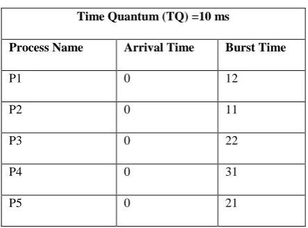
Consider five processes in ready queue with arrival time, burst time and the time quantum as shown in table 1.

Table 1: Processes specification for Case I

Time Quantum (TQ) =10 ms

Process Name Arrival Time Burst Time

P1 0 12

P2 0 11

P3 0 22

P4 0 31

P5 0 21

According to conventional Round Robin Algorithm

Fig1: Gantt chart for Round Robin in Table1

Average Waiting Time = 57.2 Average Turnaround Time =76.2 Number of Context Switches =14 According to Proposed Algorithm

Fig 2: Program output according to proposed approach

for Table 1

5.2 Case II

[image:3.595.318.540.87.251.2]

We assume that there are 5 processes in ready queue with arrival time, burst time and the time quantum as shown in table 2.

Table 2: Processes specification for Case II

P1 0 42

(4)

P3 0 82

P4 0 45

P5 0 22

[image:4.595.60.277.72.140.2]

According to Conventional Round Robin Algorithm

Fig 3: Gantt chart for Round Robin in Table 2

Average Waiting Time = 140.6 Average Turnaround Time =181.4 Number of Context Switches =15

According to Proposed Algorithm

[image:4.595.319.569.194.290.2]

Fig 4: Program output according to proposed approach for Table 2

5.3 Case III

We assume that there are 6 processes in ready queue with arrival and burst time and time quantum as shown in table 2.

Table 3: Processes specification for Case III

P1 0 11

P2 0 10

P3 0 22

P4 0 31

P5 0 25

P6 0 13

According to Conventional Round Robin Algorithm

Fig 5: Gantt chart for Round Robin in Table 3

Average Waiting Time = 65.33 Average Turnaround Time = 76.66 Number of Context Switches = 15

According to Proposed Algorithm

[image:4.595.55.300.319.415.2]

Fig 6: Program output according to proposed approach for Table 3

6. COMPARISON

OF

RESULTS

Performance of three problems stated in section 5 has been compared by considering average waiting time, average turnaround time, and number of context switches. Table 4, 5 and 6 show the result obtained whereas figure7, 8 and 9 show the comparisons.

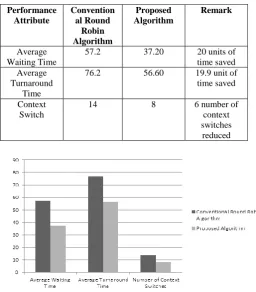
Table: 4 Computational results for Case I

Performance Attribute

Convention al Round

Robin Algorithm

Proposed Algorithm

Remark

Average Waiting Time

57.2 37.20 20 units of time saved Average

Turnaround Time

76.2 56.60 19.9 unit of time saved Context

Switch

14 8 6 number of

context switches reduced

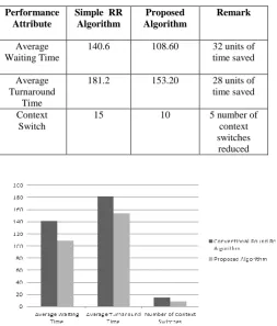
[image:4.595.304.561.440.733.2] [image:4.595.57.277.523.709.2]

(5)

[image:5.595.45.299.83.381.2]

Table: 5 Computational results for Case II

Performance Attribute

Simple RR Algorithm

Remark

140.6 108.60 32 units of time saved Average

Turnaround Time

181.2 153.20 28 units of time saved Context

Switch

15 10 5 number of

context switches

reduced

[image:5.595.50.295.432.747.2]

Fig 8: Performance Comparison for Case II

Table: 6 Computational results for Case III

Performanc e Attribute

Simple RR Algorithm

Remark

65.3 51.33 13.97 units of time saved Average

Turnaround Time

76.66 70.00 6.66 units of time saved Context

Switch

15 11 4 number of

context switches reduced

Fig 9: Performance Comparison for Case II

7. CONCLUSIONS

Time quantum plays a very important role in round robin scheduling. In this paper an improved version of round robin scheduling algorithm is proposed. This approach extends the time quantum for those processes that require only a fractional more amount of time than the allocated fixed time quantum. From the mathematical model it was proved that the worst case of the proposed algorithm is equivalent to best/worst case of conventional round robin algorithm. Experimental results also show a significant improvement in results of proposed algorithm over conventional round robin scheduling algorithm without much affecting the response time.

6. REFERENCES

[1] Rami J Matarneh. , “Self adjustment time quantum in round robin algorithm depending on burst time of the now running process”, American Journal

[2] Mohd Abdul Ahad,” Modifying round robin algorithm for process scheduling using dynamic quantum precision”, International Journal of Computer applications(0975-8887) on Issues and Challenges in Networking, Intelligence and Computing Technologies- ICNICT 2012.

[3] Saroj Hiranwal and Dr. K.C. Roy, “ Adaptive round robin scheduling using shortest burst approach based on smart time slice”, International Journal of Data Engineering, volume 2, Issue.3, 2011.

[4] Ali Jbaeer Dawood, “ Improving efficiency of round robin scheduling using ascending quantum and minimum-maximum burst time”, Journal of University of anbar for pure science : Vol. 6: No 2, 2012.

[5] Abbas Noon , Ali Kalakech and Saifedine Kadry, “ A new round robin based scheduling algorithm for operating systems: dynamic quantum using the mean average” IJCSI International Journal of Computer Science Issues, Vol. 8, Issue 3, No. 1, May 2011. [6] Pallab Banerjee, Probal Banerjee and Shweta Sonali

Dhal, “Comparative performance analysis of mid average round robin scheduling (MARR) using dynamic time quantum with round robin scheduling algorithm having static time quatum”, International Journal of Electronics and Computer Science Engineering, ISSN-2277-1956 2012.

[7] Debashree Nayak , Sanjeev Kumar Malla and Debashree Debadarshini, “Improved round robin scheduling using dynamic time quantum”, International Journal of Computer Applications (0975-8887) Volume 38- No 5, January 2012.

[8] Yaashuwanth C. & R. Ramesh, “ Intelligent time slice for round robin in real time operating system, IJRRAS 2 (2), February 2010.

[9] Braunhofer Matthias, Strumflohner Juri, “ Fair round robin scheduling”, September 17,2009.

[10]Razvan Racu, Li Li, Rafik Henia, Arne Harmann ,Rolf Ernst,” Improved Response time analysis of task scheduled under preemptive round robin, CODES+ISSS ’07,Proc of 5th

IEEE/ACM International conference on Harware/ Software codegign and system sunthesis. [11]Silberschatz, Galvin and Gagne, Operating System

Concepts, 8th edition, Wiley, 2009