Novel Approximation Algorithm for Calculating Maximum Flow in a Graph

(1)

Novel Approximation Algorithm for Calculating

Maximum Flow in a Graph

Madhu Lakshmi

Dept. of CSE

G. B. Pant Engineering College, Pauri

Uttarakhand, INDIA

Pradeep Kumar Kaushik

Dept. of CSE Uttarakhand Technical

University, Dehradun Uttarakhand, INDIA

Nitin Arora

Dept. of CSE

Women Institute of Technology, Dehradun

Uttarakhand, INDIA

ABSTRACT

In this paper a new approximation algorithm for calculating the min-cut tree of an undirected edge-weighted graph has been proposed. This algorithm runs

in

O V

(

2

.log

V V d



2

. )

, where V is the number of vertices in the given graph and d is the degree of the graph. It is a significant improvement over time complexities of existing solutions. However, because of an assumption it does not produce correct result for all sort of graphs but for the dense graphs success rate is more than 90%. Moreover in the unsuccessful cases, the deviation from actual result is very less and for most of the pairs we obtain correct values of max-flow or min-cut. This algorithm is implemented in JAVA language and checked for many input cases.

Keywords:

Maximum Flow, approximation Algorithm, complexity, min-cut tree

1. INTRODUCTION

Graph connectivity is one of the classical subjects in graph theory and has many applications like Reliability of communication networks, cluster analysis, transportation planning, chip and circuit design. Finding the minimum cut of an undirected edge-weighted graph is the fundamental algorithmic problem. Precisely it consists in finding a non-trivial partition of graph vertex set V into two parts such that the cut weight, the sum of weights of the edges connecting the two parts is the minimum. Given a graph G = (V, E) with vertex set V, edge set E and weight function w: E  R, it can be shown that there are at most n-1 distinct min-cuts among the total n(n-1)/2 pairs of nodes. We represent these n-1 min-cuts by a (not necessarily unique) tree, called Min-Cut Tree, which always exists and has the following properties [4][5][6]:

The nodes of the tree are the same as the nodes of the initial graph, (i.e. V). Each edge is assigned a value.

For every pair s, t, we can find the min-cut value by following the (unique) path between s and t in the min-cut tree. Suppose that e is the edge with minimum value

on that path. Then value (e) is also the min-cut value between s and t in the initial graph G.

To actually find the cut between s and t, we simply cut off the edge e of minimum value on the s-t path. The two connected subsets of nodes in the tree, also define the min-cut between s and t in the initial graph G.

2. WORK BACKGROUND

In the maximum flow problem we are given a flow network G = (V, E) which is a graph in which each edge (u, v)  E has a non-negative capacity

c u v

( , )



0

. If

(u, v)  E then it is assumed that

c u v

( , )



0

[1][2]. We distinguish two vertices in a flow network: a source s and a sink t. In this problem we wish to compute the greatest rate at which material can be shipped from the source s to the sink t without violating any capacity constraints.

2.1 The Max-Flow-Min-Cut theorem by

Ford and Fulkerson

The Max-Flow-Min-Cut theorem by Ford and Fulkerson [8] shows the duality of the maximum flow and minimum s-t cut. This theorem states that the value of maximum flow in a flow network G with source s and sink t is equal to the value of minimum s-t cut of G.

2.2 Gomory and Hu Algorithm

Gomory and Hu [7] showed that in a graph having n nodes, there can be only n-1 numerically different flows/cuts. They proposed a method to compute minimum-cut tree by computing only n-1 minimum s-t cuts.

2.3 M. Stoer and F. Wagner’s Algorithm

(2)

International Journal of Computer Applications (0975 – 8887) Volume 74– No.3, July 2013

3. NOVEL EFFICIENT ALGORITHM

This presents a new approximation algorithm for constructing the minimum cut tree. We calculate an upper-bound value for each node in the graph. We define the upperbound value of each node as the value of cut which separates this node from rest of the graph. We used the following Lemma:

Lemma: The value of minimum cut of a graph G separating Ni and Nj is less than or equal to minimum of

the upperbound values of two nodes Ni and Nj

We proceed by finding an edge uv such that upon merging the two nodes Nu and Nv we are able to reduce the upperbound value of the new node, i.e.

(

u

)

(

v

) 2* ( , )

upperbound N



upperbound N



w u v

max(

upperbound N

(

u

),

upperbound N

(

v

))



We start from the node having the minimum upperbound value and check for all of the edges leaving it. If we are able to reduce the upperbound value by merging it with any of the nodes, we merge the nodes and repeat the same procedure.

If we are not able to reduce the node’s upperbound value, we check for rest of the nodes in the increasing order of upperbound value.

If at any stage it is not possible to merge any node, then we merge that pair of nodes which results in minimum increment of the upperbound value.

After all the nodes in the graph are merged and it has only one node left, we proceed to construct the min-cut tree by using the information from intermediate stages.

We move from last to first stage and at each stage we see the two nodes that were merged during last stage and separate the node with smaller of the two upperbound values from the other by an arc bearing the value equal to the smaller of the two upperbound values.

Since we are considering the nodes in the increasing order of upperbound values, checking for Ni itself implies that Nj has already been checked and it was not possible to reduce its upperbound value at all. So in this

(

)

upperbound N

deviation from actual result is very less (usually for less than 5% pairs) and for most of the pairs we obtain correct values of max-flow or min-cut.

Procedure: Min-Cut Tree(G)

Input: Undirected edge-weighted graph G Output: Min-Cut Tree

Calculate the upperbound values for each node.

while(number of vertices in the current graph > 1) loop(Consider the vertices in the increasing order of upperbound value)

if(upperbound value can be reduced by merging a node with any adjacent node)

then merge those two adjacent nodes

break;

End if

End loop

if (it is not possible to merge any pair of nodes)

then merge the pair of nodes which results in minimum increment of the upperbound value.

End if End While

Construct Min-Cut Tree T by using the information from intermediate stages as described:

Move from last to first stage.

At each stage check the two nodes that were merged during last stage.

Separate the node with lower upperbound value from the other by an arc bearing the value equal to the lower upperbound value.

return T

Time Complexity of our algorithms is

2 ₂

(

.log

. )

O V

V V d



, where V is the number of vertices in the given graph and d is the degree of the graph. This is an improvement over the best existing

4

(

)

O V

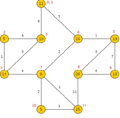
solution for minimum cut tree problem.

In the following figures we have shown the steps used in our efficient algorithm by taking some Undirected edge-weighted graph G

We start from the node having the minimum upperbound value and check for all of the edges leaving it. If we are able to reduce the upperbound value by merging it with any of the nodes, we merge the nodes and repeat the same procedure.

(3)

[image:3.595.80.278.72.272.2]

Fig. 1: Input Undirected edge-weighted graph G

[image:3.595.313.515.76.281.2]

Fig. 2: Undirected edge-weighted graph G after the first phase.

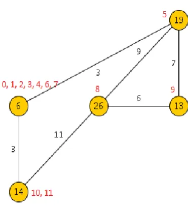
Fig. 3: Undirected edge-weighted graph G after the second phase.

[image:3.595.84.290.305.508.2] [image:3.595.315.532.347.548.2]

(4)

[image:4.595.85.528.71.534.2]

Fig. 5: Undirected edge-weighted graph G after the fourth phase.

Fig. 6: Undirected edge-weighted graph G after the

[image:4.595.322.532.75.283.2]

fifth phase

.

Fig. 7: Undirected edge-weighted graph G after the sixth phase.

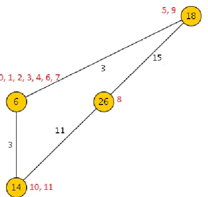
[image:4.595.322.508.317.520.2]

(5)

[image:5.595.76.283.76.271.2] [image:5.595.76.525.78.693.2]

Fig. 9: Undirected edge-weighted graph G after the eight phase.

Fig. 10: Undirected edge-weighted graph G after the

ninth phase

.

Fig. 11: Undirected edge-weighted graph G after the tenth phase.

Fig. 12: Undirected edge-weighted graph G after the eleventh phase.

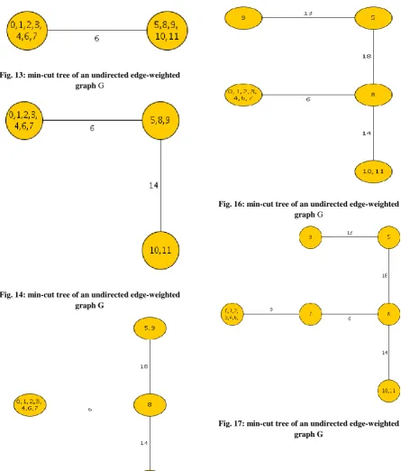
After all the nodes in the graph are merged and it has only one node left, we proceed to construct the min-cut tree by using the information from intermediate stages.

We move from last to first stage and at each stage we see the two nodes that were merged during last stage and separate the node with smaller of the two upperbound values from the other by an arc bearing the value equal to the smaller of the two upperbound values.

[image:5.595.82.284.318.517.2]

(6)

[image:6.595.76.522.71.594.2]

Fig. 13: min-cut tree of an undirected edge-weighted graph G

(7)

[image:7.595.80.537.72.537.2]

(8)

[image:8.595.76.298.74.277.2]

Fig. 22: min-cut tree of an undirected edge-weighted graph G.

4. RESULTS

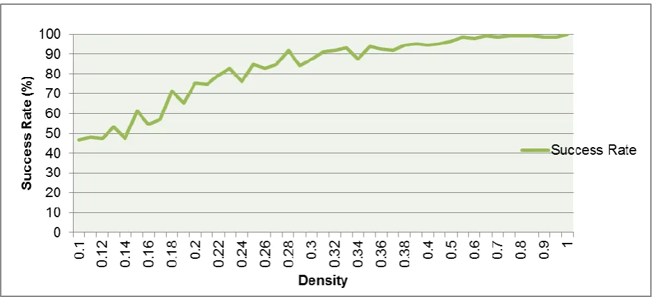
We generated 7500 random graphs of different densities but having fixed number of nodes (=50). Edge-weights

were also random and were in between 1-300. Results of running our algorithm with these graphs are summarised

in following plots:

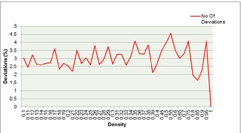
[image:8.595.72.537.402.603.2]

(9)

[image:9.595.73.546.70.328.2]

Fig 23: Plot of Deviation Vs Density (For unsuccessful test cases)

It is clear from figure 22 that for desity >= 0.4 success rate is about 100%. Figure 23 says that for the unsuccessful test cases deviation from the actual result is less than 3%. It means that even in the case of failure we get correct valus of max-flows or min-cuts for most of the pair of nodes.

4.2 Random Graphs with Random

Number of Nodes

We generated 7500 random graphs of different densities and number of nodes in them were also random (=5-55). Edges weights were also random and were in between 1-300. Results of running our algorithm with these graphs are summarised in following plots:

[image:9.595.72.542.476.690.2]

(10)

[image:10.595.72.542.69.329.2]

Fig 25: Plot of Deviation Vs Density (For unsuccessful test cases)

It is clear from figure 24 that for desity >= 0.4 success rate is more than 92%. Figure 25 says that for the unsuccessful test cases deviation from the actual result is less than 5%. It means that even in the case of failure we get correct valus of max-flows or min-cuts for most of the pair of nodes.

5. APPLICATIONS

5.1 Reliability

of

Communication

Networks:

The problem of finding the minimum cut in a graph plays an important role in the design of communication networks. An important measure of the reliability of a network is the minimum number of links that must fail in order for the communication between any pair of nodes to fail.

5.2 Cluster Analysis:

The goal of clustering is to find groups that are both homogeneous and well separated. The main idea behind using minimum cut technique for clustering is to find clusters that have small inter-cluster cuts and large intra-cluster cuts.

5.3 Transportation Planning:

The goal is to setup a network of sensors for surveillance over the complex network of roads. We find a minimum

circuit partitioning problem is closely related to the minimum cut problem.

Because of the difference between on-chip and off-chip signal delays, a good partitioning should limit the number of signals travelling off-chip to ensure high system performance.

So min-cut partitioning that minimizes the number of interconnections between different chips is desired.

6. REFERENCES

[1] Arora N., Kaushik P. K. and Singh S. P., “A Survey on Methods for finding Min-Cut Tree”. International Journal of Computer Applications (IJCA), Volume 66, No. 23, March 2013, pp. 18-22. [2] Kumar A., Singh S. P. and Arora N., “A New Technique for Finding Min-Cut Tree”. International Journal of Computer Applications (IJCA), Volume 69, No. 20, May 2013, pp. 1-7.

[3] Stoer M. and Wagner F. 1997. “A Simple Min-Cut Algorithm”. Journal of the ACM (JACM), volume 44, issue 4, 585-591.