Spurious Regression and Trending Variables

Munich Personal RePEc Archive

Spurious Regression and Trending

Variables

Noriega, Antonio E. and Ventosa-Santaulària, Daniel

Escuela de Economía, Universidad de Guanajuato, Dirección

General de Investigación Económica, Banco de México

2007

Online at

https://mpra.ub.uni-muenchen.de/58775/

Spurious Regression and Trending Variables

Antonio E. Noriega

Escuela de Economía, Universidad de Guanajuato and Dirección General de Investigación Económica, Banco de México

Daniel Ventosa-Santaulària

Escuela de Economía, Universidad de Guanajuato

School of Economics Discussion Paper EM07-1

January, 2006

JEL Classification: C12 ,C13, C22

Keywords: Spurious regression, trends, unit roots, trend stationarity, structural breaks

Abstract

This paper analyses the asymptotic andfinite sample implications of different types of nonstationary behavior among the dependent and explanatory variables in a linear spurious regression model. We study cases when the nonstationarity in the dependent and explanatory variables is deterministic as well as stochas-tic. In particular, we derive the order in probability of thet₋statistic in a lin-ear regression equation under a variety of empirically relevant data generation processes, and show that the spurious regression phenomenon is present in all cases considered, when at least one of the variables behaves in a nonstationary way. Simulation experiments confirm our asymptotic results.

1_{The authors thank Carlos Capistrán and Daniel Chiquiar for their comments. The}

opin-ions in this paper correspond to the authors and do not necessarily reflect the point of view of Banco de México. Correspondence: [email protected]

2_{Escuela de Economia, Universidad de Guanajuato. UCEA, Campus Marfil, Fracc. I,}

1

Introduction

It has been documented in recent studies that the phenomenon of spurious re-gression is present under different forms of nonstationarity in the data generating process (DGP). In particular, when the variablesyt andxtare nonstationary,

independent of each other, ordinary least squares applied to the regression model

yt=α+δxt+ut

have the following implications: 1)the OLS estimator ofδ(bδ) does not converge to its true value of zero, and2) the t-statistic for testing the null hypothesis

H0:δ= 0(teδ) diverges, thus indicating the presence of an asymptotic spurious

relationship betweenytandxt.

The rate at whichteδ diverges depends on the type of nonstationarity present

in the process generatingytandxt. In Phillips (1986), where a driftless random

walk is assumed for both variables, thet-statistic isOp(T1/2). For the case of a

random walk with drift, Entorf (1997) shows thatt_eδ diverges at rate T. More recently, Kim, Lee and Newbold (2004) (KLN henceforth) show that the phe-nomenon of spurious regression is still present even when the nonstationarity in individual series is of a deterministic nature: theyfind that, under a linear trend stationary assumption for both variables, thet-statistic isOp(T3/2). Extending

KLN’s results, Noriega and Ventosa-Santaulària (2005) (NVS hereafter), show that adding breaks in theDGP still generates the phenomenon of spurious re-gression, but at a reduced divergence rate; i.e. teδ isO(T1/2)under either single

or multiple breaks in each variable. In all these works, the implicit assumption is that both variables share the same type of nonstationarity, either stochastic (Phillips, Entorf), or deterministic (KLN, NVS).3

Although the literature on this issue has grown considerably, there are still gaps, particularly when regressions involve variables with mixed types of trend-ing mechanisms. The purpose of the present paper is tofill these gaps, using asymptotic and simulation arguments. Our results uncover the presence of spurious regressions under a wide variety of combinations of empirically rele-vant DGPs, not explored before in the literature. For instance, we consider regressions of a random walk with drift on a trend (with and without breaks)-stationary process (and vice versa). Section 2 discusses theDGPs considered. The asymptotic theory developed in Section 3 shows that the rate at which the phenomenon occurs is generallyT1/2_{, as predicted by Phillips (1998). However,}

for some combinations of trending mechanisms the divergence rate is higher. We also show that the spurious regression vanishes when one of the variables is stationary. Section 4 presents some simulation evidence forfinite samples, while Section 5 concludes.

3_{Some related papers share this same feature: Marmol (1995, 1996, 1998), Cappuccio and}

2

Trending mechanisms in the data generating

process

In a simple regression equation, the nature of the trending mechanism in the dependent and explanatory variables is unknown a priori. This is mainly due to a lack of economic knowledge on trending mechanisms. We study the spurious regression phenomenon under eight differentDGPs, widely used in applied work in economics.

We consider the following ordinary least squares regression model:

yt=αb+bδxt+ubt (1)

used as a vehicle for testing the null hypothesis H0 : δ = 0. The following

assumption summarizes the DGPs considered below for both the dependent and the explanatory variables in model (1).

Assumption_{. TheDGPs forzt=yt, xt are as follows.}

Case Name* Model 1. I(0) zt=µz+uzt

2. I(0)+br zt=µz+ PNz

i=1θizDUizt+uzt

3. TS zt=µz+βzt+uzt

4. TS+br zt=µz+ PNz

i=1θizDUizt+βzt+ PMz

i=1γizDTizt+uzt

5. I(1) ∆zt=uzt

6. I(1)+dr ∆zt=µz+uzt

7. I(1)+dr+br ∆zt=µz+ PNz

i=1θizDUizt+uzt

8. I(2) ∆2_z t=uzt

* TS,br, anddrstand for Trend-Stationary, breaks, and drift, respectively.

whereuyt anduxt are independent innovations obeying the general level

condi-tions of Assumption 1 in Phillips (1986), andDUizt,DTiztare dummy variables

allowing changes in the trend’s level and slope respectively, that is, DUizt =

1(t > Tbiz)and DTizt= (t−Tbiz)1(t > Tbiz), where1(·)is the indicator

func-tion, andTbiz is the unknown date of theith break inz. We denote the break

fraction asλiz= (Tbiz/T)∈(0,1),where T is the sample size.

Note that cases 5, 6 and 7 can be written as

zt = z0+Szt

zt = z0+µzt+Szt

zt = z0+µzt+ PMz

i=1θizDTizt+Szt

whereSzt=Pt_i=1uzi, DTizt=Pt_i=1DUizt, andz0is an initial condition.

ratios (i.e. output-capital ratio, consumption-income ratio), and the current account. Examples ofI(0)and I(0) variables with breaks have been presented in Perron and Vogelsang (1992), Wu (2000), and D’Adda and Scorcu (2003). Cases 3 to 8 are widely used to model growing variables, real and nominal, such as output, consumption, money, prices, etc. Macro variables have been described asI(0)around a linear trend,I(0)around a linear trend with structural breaks, andI(1)in Perron (1992, 1997), Lumsdaine and Papell (1997), Mehl (2000), and Noriega and de Alba (2001). Combinations of case 8 with other cases are often behind the empirical modelling of nominal specifications expressed in terms of I(2) (nominal) and I(1) or I(0)+breaks (real) variables. Economic models involvingI(2)variables include models of money demand relations, purchasing power parity, and inflation and the markup. Examples of variables described as I(2) can be found in Juselius (1996, 1999), Haldrup (1998), Muscatelli and Spinelli (2000), Coenen and Vega (2001), and Nielsen (2002).

TheDGPs include both deterministic and stochastic trending mechanisms, with 49 possible nonstationary combinations of them among the dependent and the explanatory variables, where case 1 is included as a benchmark.4

The spurious regression phenomenon has already been analyzed for a few combinations ofDGPs in the Assumption. For instance, the case of both vari-ables following a unit root (case 5) was studied by Granger and Newbold (1974) and Phillips (1986), and case 6 by Entorf (1997). The case (3) of a trend-stationary model for both variables was studied by Hassler (2000) and KLN, while its extension to multiple breaks (case 4) by NVS. Mixtures of integrated processes were studied by Marmol (1995), who considers cases 5 and 8 (y fol-lows a unit root, whilexfollows two unit roots, and vice versa). Many other combinations, however, have not been analyzed. Among them, combinations 3-6 and 4-6, which have practical importance, given the empirical relevance of structural breaks in the time series properties of many macro variables.

3

Asymptotics for spurious regressions

This section presents the asymptotic behavior of thet-statistic for testing the null hypothesisH0:δ= 0(teδ) in model (1) when the dependent and explanatory

variables are generated according to combinations ofDGPs in the Assumption. In the following Theorem, which collects the main results, a combination of DGPs is indicated by the pair i₋j, (i, j = 1,2, ...,8) indicating thatyt is

generated by casei, whilextby casej, both defined in the Assumption. Thus,

for instance, the combination 8₋5corresponds to model (1) whereyt isI(2)

(case8), whilextisI(1)(case5).

4_{We do not consider the cases of I(1) processes with long memory errors, and fractionally}

Theorem_{. The order in probability of te}

δ in model (1) depends on the

combi-nation of DGPs for yt and xt in the Assumption, as follows:

a) t_eδ =Op(1) for combination of cases 1−iand i−1, i= 1,2, ...,8;

b) t_eδ =Op(T1/2) for combination of cases i−i, i= 2,4,5,7,8,

and i₋j;i, j= 2,3, ...,8;i6=j;

except for combinations 3₋3,3₋6,6₋3and 6₋6; c) teδ =Op(T) for combination of cases 3−6,6−3and 6−6;

d) teδ =Op(T3/2) for combination of cases 3−3.

Proof_{. Combination 1-1 represents the classical textbook situation, in which}

the t-statistic converges to a standard normal distribution (see for instance White (1984, Chapter V)). Results for combinations 1-2, 2-1, and 2-2 are special cases of Hassler (2003), while 3-3 comes from Hassler (2000) and KLN (who also studied the case 1-3 and 3-1); for 4-4, 5-1, 5-5, 6-6, 8-8, and 5-8 results come from NVS, Hassler (1996), Phillips (1986), Entorf (1997), Marmol (1995), and Marmol (1996), respectively. The proof for the remaining 51 combinations was assisted by the softwareMathematica, and, since the mechanics for obtaining the order in probability is the same for each combination ofDGPs, we only present the procedure for a single combination, discussed in the Appendix at the end of the paper.

Part a) indicates that when either both variables are I(0), or one of the variables is I(0) while the other follows any of the other nonstationary cases, the spurious regression phenomenon is not present, since the t-statistic does not diverge to infinite; instead, it converges (to a constant, or to a random variable, depending on theDGPs.) For the majority of combination of cases, thet−statistic diverges (at rate√T or faster), indicating a spurious relationship among independent variables, as partsb)-d) show.

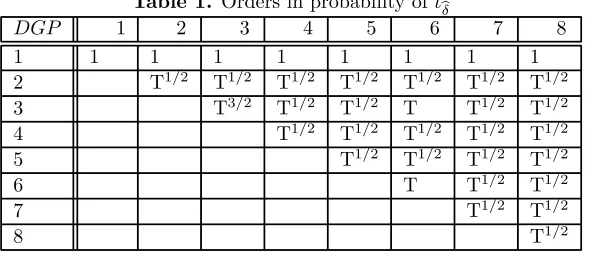
Table 1 summarizes the abovefindings. The symmetry of results imply that the order in probability does not depend on the type of nonstationarity among dependent and explanatory variables.

Table 1. Orders in probability oft_eδ

DGP 1 2 3 4 5 6 7 8

1 1 1 1 1 1 1 1 1

2 T1/2 _T1/2 _T1/2 _T1/2 _T1/2 _T1/2 _T1/2

3 T3/2 _T1/2 _T1/2 _{T T}1/2 _T1/2

4 T1/2 _T1/2 _T1/2 _T1/2 _T1/2

5 T1/2 _T1/2 _T1/2 _T1/2

6 T T1/2 _T1/2

7 T1/2 _T1/2

Therefore, when two independent random variables follow any of the nonsta-tionary combinations considered in the Assumption, OLS inference will indicate, asymptotically, a significant (spurious) relationship among them.

The representation theory developed by Phillips (1998) shows that a trend-ing stochastic (or deterministic) process can be represented in various ways. In particular, it can be written as an infinite linear combination of trending deter-ministic (stochastic) functions with random coefficients. In such an asymptotic environment, he shows that the regressiont-ratios of the fitted coefficients di-verge at rate√T. Results from the theorem above indicate that relatively simple nonstationary time series models correctly indicate the presence of the limiting representation.5

4

Experimental results

We computed rejection rates of the t-statistic for testing the null hypothesis

H0 : δ= 0, in model (1), using a 1.96 critical value (5% level) for a standard

normal distribution. In order to assess the usefulness for a finite sample of the asymptotic results presented in the theorem, rejection rates were based on simulated data, for samples of sizeT = 25,50,100,250,500,1,000,and10,000, under various combinations ofDGPs in the Assumption.6 _{In all experiments,}

the number of replications is 10,000.

Table 2. Rejection Rates forteδ; the case of two breaks

Combinations of cases (DGPs) in the Assumption

T 1-7 2-2 2-4 2-6 3-4 3-6 4-4 4-6 4-7 4-8 6-8 7-8 25 .06 .34 .62 .81 .14 .25 .32 .61 .66 .65 .93 .94 50 .06 .57 .96 .99 .89 .95 .99 .99 .99 .94 .95 .96 100 .05 .87 1.0 1.0 1.0 .99 1.0 1.0 1.0 .97 .97 .97 250 .05 1.0 1.0 1.0 1.0 1.0 1.0 1.0 1.0 .98 .98 .98 500 .06 1.0 1.0 1.0 1.0 1.0 1.0 1.0 1.0 1.0 1.0 1.0 1000 .05 1.0 1.0 1.0 1.0 1.0 1.0 1.0 1.0 1.0 1.0 1.0

The values of the parameters in theDGPs are as follows: σz = 1, φz = 0, µx = 0.4,

µ_y= 0.7,β_x= 0.07,β_y= 0.04,θxi= 0.07,θyi= 0.04,γxi= 0.02,γyi= 0.04, for

i= 1, ...Mz,Mz = 2, forz =x, y. Breaks inx(y) occur at 20% (40%) and 70% (80%)

of total data length.

5_{The cases of linear deterministic trends without breaks (combinations 3-3, 3-6 and 6-6) do}

notfit in the general framework ofT1/2 _{divergence of Phillips (1998). This is because these}

cases are not truly spurious, since the limit value ofeδin (1) is not zero, but the ratio of the linear trend parameters in the DGP. On this issue see Hassler (2000) and KLN.

6_{The experimental results in this section are limited, and only serve as a guide on thefinite}

Table 3. Rejection Rates forteδ; the case of four breaks

Combinations of cases (DGPs) in the Assumption

T 1-7 2-2 2-4 2-6 3-4 3-6 4-4 4-6 4-7 4-8 6-8 7-8 25 .06 .44 .68 .83 .54 .25 .63 .89 .82 .79 .93 .96 50 .05 .67 .98 .99 .97 .95 .99 .99 .99 .94 .95 .99 100 .05 .91 1.0 1.0 1.0 .99 1.0 1.0 1.0 .97 .97 1.0 250 .06 1.0 1.0 1.0 1.0 1.0 1.0 1.0 1.0 .98 .98 1.0 500 .05 1.0 1.0 1.0 1.0 1.0 1.0 1.0 1.0 1.0 1.0 1.0 1000 .05 1.0 1.0 1.0 1.0 1.0 1.0 1.0 1.0 1.0 1.0 1.0

Experimental design as above, but withMz = 4, forz =x, y. Breaks in x(y) occur at

15% (20%), 30% (35%), 50% (55%) and 70% (80%) of total data length.

Tables 2 and 3 present rejection rates under 12 different combinations of

DGPs in the Assumption. In Table 2, the cases where breaks are considered (all but 3-6 and 6-8) include 2 breaks, while Table 3 presents results when 4 breaks are allowed. The column labeled 1-7 in both tables presents thefinite sample counterpart of the Op(1) result in parta)of the theorem: thet-statistic does not

diverge, indicating that the spurious regression phenomenon is not a problem infinite samples. For the rest of cases, the asymptotic nonsense relationship reported in the theorem is also detected in our simulation experiments: the spurious regression phenomenon is present even for samples as small as 25. In comparing results from Tables 2 and 3, it can be noted that a nonsense regression is more likely when the number of structural breaks increases in theDGP.

5

Conclusions

This paper has presented an asymptotic and experimental analysis of the spu-rious regression phenomenon under a wide variety of empirically relevant data generating processes in a simple regression model. Itfills many gaps left open by previous research in the area. In particular, it shows that thet-statistic for testing a linear relationship among independent time series diverges, if both variables show a nonstationary behavior, due to either stochastic (unit roots) or deterministic (linear trends and/or structural breaks) factors.

Our results particularize Phillips’ (1998) general results to empirically use-ful models, by showing that the phenomenon of spurious regression is present for time series with relatively simple trending mechanisms. This phenomenon depends on the commonality of trends and/or breaks in both dependent and explanatory variables. If the nonstationary behavior (stochastic or determin-istic) is present in only one of the variables, however, the spurious regression vanishes. Our simulation experiments reveal that a spurious regression is not exclusively an asymptotic phenomenon, it will also be present infinite samples for the majority ofDGPs considered.

analysis: the probability offinding a nonsense correlation among independent series will not only be high infinite samples, but it will grow with the sample size.

6

Appendix

We present a guide on how to obtain the order in probability of one combination ofDGPs, namely, the combination 1-7, for which

yt=µy+uyt

xt=x0+µxt+ PMx

i=1θixDTixt+Sxt

The orders in probability for the rest of cases follow the same steps. The proofs were assisted by the softwareMathematica 4.1. The corresponding codes for all combinations ofDGPs are available at www.ventosa-santaularia.com/NVS_06a.zip. Below, we describe the steps involved in the computerized calculations.

Write the regression modelyt=α+δxt+utin matrix form: y=Xβ+u. The

vector ofOLSestimators isβb= (αb bδ)0_{= (X}0_X)−1_X0_{y, and thet-statistic of}

interestteδ=bδ h

b

σ2_u(X0_X)−1 22

i−1/2

, where(X0_X)−1

22 is the2nddiagonal element of

(X0_X)−1 _andbσ2 u=T−1

PT

t=1ub2t =T−1 PT

t=1 ³

yt−αb−bδxt ´2

. t_eδ is a function of the following objects:

T P t=1

yt=µyT+ΣuyT1/2 T P t=1 y2 t = ¡ µ2

y+Σu2y¢T+ 2µyΣuyT1/2 T

P t=1

xt=1₂

∙

µ_x+MxP i=1

θi(1−λi)2 ¸

T2_+Σ

sxT3/2+

∙

x0+1₂ µ

µ_x+MxP i=1

θi(1−λi) ¶¸ T T P t=1 x2 t = ∙ 1

3µ2x+λ++13µx Mx_P

i=1

θi(1₋λi)2_(λ i+ 2)

¸

T3_{+2 (µ}

xΣtsx+Σts1xi)T5/2 +Op(T2)

T P t=1

ytxt= h

1

2µy(µx+ PMx

i=1θi(1−λi)2) i

T2_+Op(T3/2₎

with

Σuy =T−1/2PTt=1uyt

Σu2y =T−1PTt=1u2yt

Σsx =T−3/2PTt=1Sxt

Σtsx=T−5/2PTt=1tSxt

Σts1xi=T−5/2PMxi=1θi³PTt=T_bi+1tSxt−λiPTt=T_bi+1Sxt ´

λ+= 1 3

PMx

i=1θ2i(1−λi)2+ Mx_P−1

i=1 Mx_P

j=i+1

θiθj £₂

3(1−λu(i,j))3+λd(i,j)(1−λu(i,j))2 ¤

λl(i,j)= min(λi, λj)

λd(i,j)=λu(i,j)−λl(i,j)

where (see for instance Phillips (1986)),

Σuy ⇒σyWy(1)

Σu2y ⇒σ2y

Σsx ⇒σx R1

0 Wx(r)dr

Σtsx⇒σx R1

0 rWx(r)dr

Σts1xi⇒σxPMxi=1θi R1

λi(r−λi)Wx(r)dr,

⇒ signifies convergence in distribution, and Wz(r), z = y, x is the standard

Wiener process onr_∈[0,1].

Using these expressions,Mathematicacomputes the limiting distribution of the parameter vector and the rest of the elements oft_eδ by factoring out the relevant expressions in powers of the sample size. In this way, the orders in probability can be determined, and the limiting expression obtained, by retaining only the asymptotically relevant terms, upon a suitable normalization. From Mathemat-ica’s output it can be deduced that, for the case at hand,

T3/2_bδh_bσ2

uT3(X0X)−221 i−1/2

=bδhσb2_u(X0_X)−1 22

i−1/2

=Op(1),

as reported in the Theorem.

7

References

Cappuccio, N. and D. Lubian (1997), "Spurious Regressions BetweenI(1)

Processes with Long Memory Errors", Journal of Time Series Analysis, 18, 341-354.

Coenen, G. and J.-L. Vega (2001), "The Demand for M3 in the Euro Area",

Journal of Applied Econometrics, 16, 727-48.

D’Adda, C. and A. E. Scorcu (2003), "On the Time Stability of the Output-Capital Ratio",Economic Modelling, 20, 1175-1189.

Entorf, H. (1997), "Random Walks with Drifts: Nonsense Regression and Spurious Fixed-Effect Estimation",Journal of Econometrics, 80, 287-296.

Granger, C.W.J. and P. Newbold (1974), "Spurious Regression in Econo-metrics",Journal of Econometrics, 2, 111-120.

Granger, C.W.J., N. Hyung, and Y. Jeon (1998), "Spurious Regressions with Stationary Series", Mimeo.

Haldrup, N. (1998), "An Econometric Analysis of I(2)Variables", Journal of Economic Surveys, 12(5), 595-650.

Hassler, U. (1996), "Spurious Regressions when Stationary Regressors are Included",Economics Letters, 50, 25-31.

______ (2000), "Simple Regressions with Linear Time Trends", Journal of Time Series Analysis, 21, 27-33.

Juselius, K. (1996), "A Structured VAR under Changing Monetary Policy",

Journal of Business and Economic Statistics, 16, 400-12.

Juselius, K. (1999), "Price Convergence in the Medium and Long Run: An

I(2)Analysis of Six Price Indices", in Engle, R. F. and H. White (eds.): Coin-tegration, Causality and Forecasting. A Festschrift in Honour of Clive W. J. Granger, Oxford University Press.

Kim, T.-H., Y.-S. Lee and P. Newbold (2004), "Spurious Regressions with Stationary Processes Around Linear Trends",Economics Letters, 83, 257-262.

Lumsdaine, R.L. and D.H. Papell (1997), ”Multiple Trend Breaks and the Unit Root Hypothesis”,The Review of Economics and Statistics, 79, 212-218.

Marmol (1995), "Spurious Regressions forI(d)Processes",Journal of Time Series Analysis, 16, 313-321.

Marmol, F. (1996), "Nonsense Regressions Between Integrated Processes of Different Orders",Oxford Bulletin of Economics and Statistics, 58(3), 525-36.

Marmol, F. (1998), "Spurious Regression Theory with Nonstationary Frac-tionally Integrated Processes",Journal of Econometrics, 84, 233-50.

MATHEMATICA 4.1 (2000), Wolfram Research Inc.

Mehl, A. (2000), "Unit Root Tests with Double Trend Breaks and the 1990s Recession in Japan",Japan and the World Economy, 12, 363-379.

Muscatelli, V. A. and F. Spinelli (2000), "The Long-Run Stability of the Demand for Money: Italy 1861-1996", Journal of Monetary Economics, 45, 717-39.

Nielsen, H. B. (2002), "An I(2) Cointegration Analysis of Price and Quantity Formation in Danish Manufactured Exports",Oxford Bulletin of Economics and Statistics, 64(5), 449-72.

Noriega, A. and E. de Alba (2001), "Stationarity and Structural Breaks: Evidence from Classical and Bayesian Approaches", Economic Modelling, 18, 503-524.

Noriega, A. and D. Ventosa-Santaulària (2005), "Spurious Regression Under Broken Trend Stationarity", Working Paper EM-0501, School of Economics, University of Guanajuato. Forthcoming inJournal of Time Series Analysis.

Park, J. Y. and P. C. B. Phillips (1989), "Statistical Inference in Regressions with Integrated Processes: Part 2",Econometric Theory, 5, 95-131.

Perron, P. (1992), "Trend, Unit Root and Structural Change: A Multi-Country Study with Historical Data", inProceedings of the Business and Eco-nomic Statistics Section, American Statistical Association, 144-149.

Perron, P. (1997), "Further Evidence on Breaking Trend Functions in Macro-economic Variables",Journal of Econometrics, 80, 355-385.

Perron, P. and T. J. Vogelsang (1992), "Nonstationarity and Level Shifts with and Application to Purchasing Power Parity", Journal of Business and Economic Statistics, 10(3), 301-20.

Perron, P. and X. Zhu (2005), "Structural Breaks with Deterministic and Stochastic Trends",Journal of Econometrics, 129, 65-119.

Phillips, P.C.B. (1998), "New Tools for Understanding Spurious Regres-sions",Econometrica, 66(6), 1299-1325.

Tsay, W.-J. and C.-F. Chung (1999), "The Spurious Regression of Fraction-ally Integrated Processes", Mimeo.