Proceedings of the 12th International Workshop on Semantic Evaluation (SemEval-2018), pages 990–994
BomJi at SemEval-2018 Task 10:
Combining Vector-, Pattern- and Graph-based Information
to Identify Discriminative Attributes
Enrico Santus1, Chris Biemann2, Emmanuele Chersoni3 [email protected],
[email protected], [email protected]
1Massachussetts Institute of Technology, 2 Universit¨at Hamburg,
3Aix-Marseille University
Abstract
This paper describes BomJi, a supervised sys-tem for capturing discriminative attributes in word pairs (e.g. yellowas discriminative for
bananaover watermelon). The system relies on an XGB classifier trained on carefully engi-neered graph-, pattern- and word embedding-based features. It participated in the SemEval-2018 Task 10 on Capturing Discriminative At-tributes, achieving an F1 score of 0.73 and
ranking 2nd out of 26 participant systems.
1 Introduction
The recent introduction of popular software packages for training neural word embeddings
(Mikolov et al., 2013a,b; Levy and Goldberg, 2014) has led to an increase of the number of stud-ies dedicated to lexical similarity and to remark-able performance improvements on related tasks (Baroni et al.,2014).
However, the validity of similarity estimation as the only benchmark for semantic representa-tions has been questioned, for several reasons. One for all, most evaluation datasets provide human-elicited similarity scores, with the conse-quences that the ratings are subjective and the performance of some automated systems is al-ready above the upper bound of the inter-annotator agreement (Batchkarov et al.,2016;Faruqui et al., 2016;Santus et al.,2016a).
Originally proposed as an alternative bench-mark for Distributional Semantic Models (DSMs), the Discriminative Attributes task focuses in-stead on the extraction of semantic differences
between lexical meanings (Krebs and Paperno, 2016): given two words and an attribute (i.e., a discrete semantic feature), a system has to pre-dict whether the attribute describes a difference between the corresponding concepts or not (e.g.
wingis an attribute ofplane, but not ofhelicopter).
Since even related words may differ for some non-shared attributes (e.g. hypernyms and hy-ponyms), the ability of automatically recognize discriminative features would be an extremely useful addition for the creation of ontologies and other types of lexical resources and would make machine decisions interpretable, enabling human validation (Biemann et al.,2018). Moreover, one can think to applications to many other NLP do-mains, such as machine translation and dialogue systems (Krebs and Paperno,2016).
In the present contribution, we describe the BomJi classification system, which we used for the identification of discriminative features be-tween concept pairs. According to the official evaluation results provided by the organizers1, our
system ranked second out of 26 participants. Our score, F1 = 0.73 lags slightly behind the best score of0.75. After the evaluation period, we run further experiments including all investigated fea-tures and found that the system can achieve up to 0.75F1 score.
2 Capturing Discriminative Attributes
2.1 Task and Dataset Description
The task of capturing discriminative attributes be-tween words can be described as a binary classi-fication task, in which the system has to assign a positive label if the feature is discriminative for the first concept over the second one, and a negative label otherwise.
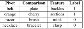
In the test data, the first two words correspond to the concepts being compared (they are called, re-spectively, thepivotand thecomparisonterm) and the third word is the feature, which could describe a discriminative attribute or not (some examples are shown in Table 1). In the paper, we will refer
1https://competitions.codalab.org/
competitions/17326#results
Pivot Comparison Feature Label belt plate buckles 1 orange cherry sections 1
razor brush mink 0
[image:2.595.112.253.62.111.2]necklace bracelet clasp 0
Table 1: Examples of triples from the training dataset.
Dataset Examples Features Split P-N Training 17,782 1,292 37.06%-62.94% Validation 2,722 576 50.1%-49.9%
Test 2,340 577 44.74%-55.26%
Table 2: Number of examples, distinctive features and Positive-Negative split for each dataset.
to the elements of the triples asw1,w2andf eat.
A training and validation set have been provided for system development (figures in Table 2).
2.2 Embeddings and Graphs
For the Discriminative Attributes task, we com-bined word embeddings, patterns and information extracted from a graph-based distributional model. Concerning the word embeddings, we used the vectors produced by two popular frameworks for word embeddings: Word2Vec (Mikolov et al., 2013a,b) and GloVe (Pennington et al., 2014).2
The Word2Vec Skip-Gram architecture is a single-layer neural network, based on the dot-product be-tween word vectors, in which the vector represen-tation is optimized to predict the context of a tar-get word given the word itself. The context gen-erally consists of a word window of a fixed width around the target. The other framework, GloVe, is similar to traditional count models based on ma-trix factorization (Turney and Pantel,2010;Baroni et al.,2014), in the sense that vectors are trained on global word-word co-occurrence counts. In the case of GloVe, the training objective is to learn word vectors such that their dot product equals the logarithm of the probability of the word to co-occur (Pennington et al.,2014).
As for graph-based information, we used the Jo-BimText architecture introduced byBiemann and Riedl(2013). In JoBimText, lexical items are rep-resented as the set of theirpmost salient contexts,
where the contexts are words connected to the tar-get by a given syntactic link or by a lexical pattern, and saliency is defined as an association measure
2The pre-trained vectors are available, respectively,
at https://code.google.com/archive/p/ word2vec/ (Google News, 300 dimensions) and at https://nlp.stanford.edu/projects/glove/ (Common Crawl, 840B tokens, 300 dimensions).
between target and context, such as Positive Lo-cal Mutual Information (Evert,2004). Differently from vector models, similarity between words in JoBimText is simply based on the overlap count of their common contexts.
Regarding patterns, first we extracted sentences where words and their features co-occur from a web-scale sentence-based index of English web (Panchenko et al.,2018) and then we extracted the patterns connecting our target words.
2.3 Methodology
The predictions submitted for the evaluation of Task 10 were obtained with a system that consists of a classifier, the Extreme Gradient Boosting (or XGBoost,Chen and Guestrin (2016)), trained on vectors aggregating carefully engineered graph-, pattern- and word embedding features.
In this section, we provide an overview of each feature type, leaving the discussion of their contri-bution to Section3. The total of 55,026 features we used can be divided into five major groups.
CO-OCCURRENCE. Thirteen features re-lated to word and word-feature frequency were calculated on the basis of the information ex-tracted from a corpus of3.2B words,
correspond-ing to about 20% of the Common Crawl. For each word-feature combination (i.e. w1 − f eat and
w2−f eat), we calculated: i) the co-occurrence
count; ii) word count; iii) feature count; iv) Posi-tive Pointwise Mutual Information (PPMI (Church and Hanks,1990)) between each word and the fea-ture; v) Positive Local Mutual Information (PLMI (Evert,2004)) between each word and the feature. Further, we added three features representing the subtractions between the values of i), iv) and v) for the two word-feature combinations.
JOBIMTEXT.Another set of twenty-four fea-tures comes directly from JoBimText. They were calculated after extracting information through the public accessible JoBimText API3, which
re-turns a JSON file containing - for every tar-get - a sorted list of N features and their
as-sociation scores (up to N = 1,000). As Jo-BimText distinguishes features according to their POS and dependency roles (i.e. features are in form WORD#POS#DEPENDENCY), a given
f eatmay appear multiple times in different
POS-dependency combinations. However, we found that f eat rarely appears in the top N features
[image:2.595.89.278.143.184.2]ofw1 andw2, so we calculated our features not only for the given targets (i.e. wx), but also
for the first among their top 10 neighbors for whichf eatwas found (i.e. top(neighbor(wx) 3 f eat, max= 10)) and the first among the top 10
f eatneighbors for which the target was found (i.e. top(neighbor(f eat) 3wx, max= 10)). This
al-lowed us to check also whether the neighbors of the given words were associated with the candi-date discriminative attributes or vice versa. The features are defined as follows (here they are de-scribed only with reference to the query on wx,
but this should be generalized to the other cases):
• prediction by rank: it is1iff eatis ranked higher for
w1than forw2,0otherwise;
• prediction by score: it is1if the total score between
w1−f eatis higher than forw2−f eat,0otherwise; • total score: sum of the scores ofw1−f eatif prediction
by score is1, ofw2−f eatotherwise;
• top rank: top rank off eatforw1if prediction by score
is1, forw2otherwise;
• bottom rank: last rank off eatforw1if prediction by
score is1, forw2otherwise;
• number of occurrences: count of how many times a feature appears among the features ofw1if prediction
by score is1, otherwise the occurrences among the fea-turesw2are counted;
• which neighbor?: integer showing whether the query was performed onw1/w2(in this case it would be ini-tialized to0), or on its neighbors (in this case it would be initialized with the rank of the first neighbor where
f eatwas found);
• whichf eatneighbor?: integer showing whether the query was performed onw1/w2(in this case it would be initialized to0) or on thef eatneighbors (in this case it would be initialized with the rank of the first
f eatneighbor wherew1orw2was found).
WORD EMBEDDING FEATURES.Mikolov et al. (2013a) showed how vector offsets encode semantic information. We decided to include five features computed from either the Word2Vec or the Glove vectors, in order to take advantage of the offset information.
They are computed, respectively, as:cos((w1−
w2), f eat), cos((w1 − f eat),(w2 − f eat)),
cos((w1−f eat), w2),cos((w2−f eat), w1). Fi-nally, also the cosine between the word vectors (i.e. cos((w1, w2)) has been included.
WORD EMBEDDING VECTORS. These features are the simple concatenation of the three vectors ofw1,w2andf eat. Again, we have two
versions of these features, one for Word2Vec and one for Glove.
PATTERNS.In order to characterize the rela-tion between words and features, we used an index to extract patterns occurring between them, inde-pendently of the order in which they appeared, and limited the maximum number of results to 10,000 sentences.
The patterns consist of sequences of either lem-matized tokens, POS or dependency tags, which are used to abstract from the surface form, thereby increasing the recall. Since the number of ex-tracted patterns was far too high, we decided to use only patterns with a frequency higher than 100, obtaining a set of 53,136 items, using the observed pattern frequency per word pair as a predictor.
3 Experiments
3.1 Choosing the Training Set
During the practice phase, we noticed that the training set and the validation set show very differ-ent distributions. Running 5-fold cross validation experiments on either dataset, we obtained very high scores (sometimes close to0.95). However, such scores did not generalize to the other dataset, where they dropped to about0.60.
This was only partially due to lexical memo-rization (some lexemes were present in multiple triples of the same dataset, cf. Levy et al.(2015); Santus et al. (2016b)). In fact, investigating the frequency of the words in the triples, we found that, on average, in our index, the first and the second words,w1andw2, were about four times more frequent in the validation than in the train-ing set (respectively4.7Mand5.4Mversus0.9M
and 1M); similarly, the third word (i.e. f eat)
was almost twice more frequent in the validation than in the training set (i.e. 3.9M versus2.9M). When the test set was made available, we could verify that its frequency distribution resembled the one in the validation set, with the first and second words respectively at3.3M and2M, and the third
at about4.5M occurrences.
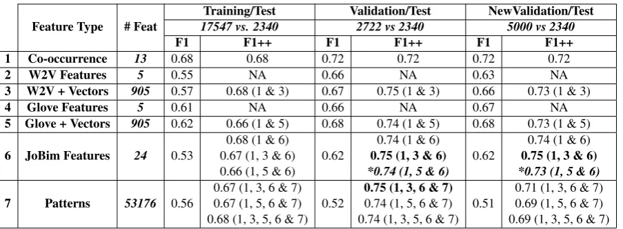
Feature Type # Feat 17547 vs. 2340Training/Test Validation/Test2722 vs 2340 NewValidation/Test5000 vs 2340
F1 F1++ F1 F1++ F1 F1++
1 Co-occurrence 13 0.68 0.68 0.72 0.72 0.72 0.72
2 W2V Features 5 0.55 NA 0.66 NA 0.63 NA
3 W2V + Vectors 905 0.57 0.68 (1 & 3) 0.67 0.75 (1 & 3) 0.66 0.73 (1 & 3)
4 Glove Features 5 0.61 NA 0.66 NA 0.67 NA
5 Glove + Vectors 905 0.62 0.66 (1 & 5) 0.68 0.74 (1 & 5) 0.68 0.73 (1 & 5) 6 JoBim Features 24 0.53 0.67 (1, 3 & 6)0.68 (1 & 6)
0.66 (1, 5 & 6) 0.62
0.74 (1 & 6) 0.75 (1, 3 & 6)
*0.74 (1, 5 & 6) 0.62
0.74 (1 & 6) 0.75 (1, 3 & 6)
*0.73 (1, 5 & 6)
7 Patterns 53176 0.56 0.67 (1, 3, 6 & 7)0.67 (1, 5, 6 & 7) 0.68 (1, 3, 5, 6 & 7) 0.52
0.75 (1, 3, 6 & 7) 0.74 (1, 5, 6 & 7) 0.74 (1, 3, 5, 6 & 7) 0.51
[image:4.595.76.528.60.226.2]0.71 (1, 3, 6 & 7) 0.69 (1, 5, 6 & 7) 0.69 (1, 3, 5, 6 & 7) Table 3: Results both in absolute (F1) and in incremental terms (F1++: in brackets the features used to obtain the score) on the test set, organized by training set. In bold, we report the best results. In bold-italics, we report the submitted systems.
total of 5,000 samples. The use of different train-ing data was the only difference between the two submissions.
3.2 Model Selection
During the practice phase, we performed ex-periments with several classifiers, including K-Neighbors (with K = 3), Decision Tree (with max depth = 5), Random Forest (with
max depth = 5, n estimators = 10 and
max f eatures= 1), Multilayer Perceptron (with
alpha = 1), AdaBoost and XGB (the latter two with default settings).
Before running the classifiers, we also used Linear Support Vector Classification (SVC) with
penalty =0 l10 and we tested several values ofC
(i.e. 0.05,0.1,0.25,0.5,1) for feature selection. In almost all settings we found that the best per-forming classifiers were the Random Forest, the Multilayer Perceptron and, above all others, XGB. With respect to the value ofC for the feature
se-lection, instead, we noticed that it varied in rela-tion to the feature types, with minor influence on the performance of XGB (+/-2%). In the final sub-mission, therefore, we opted for removing this step from the pipeline and for keeping the full vector.
Concerning feature selection, we found that the pattern features had a neutral effect on the perfor-mance during cross validation. Similarly we no-ticed that Glove and Word2Vec performed compa-rably. Thus, we opted for submitting the output of the systems without using the pattern features and only Glove features (Word2Vec had lower cover-age on the dataset). As it can be noticed in Table 3, however, this decision has slightly lowered the
performance of our system in the competition.
3.3 Feature Contribution
In order to measure the contribution of the fea-tures, we re-ran the experiments over the test set, after training our model on the three available sets: training, validation and new validation sets.
Results are reported in Table 3, in which it is easy to notice a few things: the performance is strongly related to the choice of the training set, with Validation being better that New Validation, which is in turn better than the original Training set; the thirteen co-occurrence features are those that provide the major contribution to the perfor-mance, reaching a F1 score of 0.72. Further useful features are the word embedding vectors (900 fea-tures), the word embedding features (5 features) and, to some extent, the information from JoBim-Text. Pattern-based features perform the worst, al-most on par with random guessing.
The submitted systems do not correspond to the systems obtaining the best performance in post-evaluation experiments (see the bold and bold-italics scores in Table 3); this was due to the use of Glove instead of Word2Vec in our submitted sys-tems, because none of the embedding models had an edge over the other in the validation process.
4 Conclusions
graph-, pattern- and word embedding-based fea-tures. In the paper we have reported the contribu-tion for each features, discussing the model selec-tion and showing that a major factor affecting the performance was the choice of the training data.
In the official Task 10 evaluation, our submitted systems achieved an F1 score of0.73, ranking 2nd out of 26 participant systems.
References
Marco Baroni, Georgiana Dinu, and Germ´an Kruszewski. 2014. Don’t Count, Predict! A Systematic Comparison of Context-Counting
vs. Context-Predicting Semantic Vectors. In
Proceedings of ACL, pages 238–247.
Miroslav Batchkarov, Thomas Kober, Jeremy Reffin, Julie Weeds, and David Weir. 2016. A Critique of Word Similarity as a Method for Evaluating Distri-butional Semantic Models. InProceedings of the 1st Workshop on Evaluating Vector-Space Representa-tions for NLP, pages 7–12.
Chris Biemann, Stefano Faralli, Alexander Panchenko, and Simone Paolo Ponzetto. 2018. A Framework for Enriching Lexical Semantic Resources with
Dis-tributional Semantics. Natural Language
Engineer-ing, 24(2):265–312.
Chris Biemann and Martin Riedl. 2013. Text: Now in 2D! A Framework for Lexical Expansion with Con-textual Similarity. Journal of Language Modeling, 1(1):55–95.
Tianqi Chen and Carlos Guestrin. 2016. XGBoost: A
Scalable Tree Boosting System. InProceedings of
the 22nd ACM Sigkdd International Conference on Knowledge Discovery and Data Mining, pages 785– 794.
Kenneth W. Church and Patrick Hanks. 1990. Word Association Norms, Mutual Information, and Lexi-cography.Computational Linguistics, 16(1):22–29.
Stefan Evert. 2004. The Statistics of Word Cooccur-rences: Word Pairs and Collocations. Ph.D. thesis.
Manaal Faruqui, Yulia Tsvetkov, Pushpendre Rastogi, and Chris Dyer. 2016. Problems With Evaluation
of Word Embeddings Using Word Similarity Tasks.
In Proceedings of the 1st Workshop on Evaluating Vector-Space Representations for NLP, pages 30– 35.
Alicia Krebs and Denis Paperno. 2016. Capturing Discriminative Attributes in a Distributional Space:
Task Proposal. In Proceedings of the 1st
Work-shop on Evaluating Vector-Space Representations for NLP, pages 51–54.
Omer Levy and Yoav Goldberg. 2014. Neural Word Embedding as Implicit Matrix Factorization. In Ad-vances in Neural Information Processing Systems 27, pages 2177–2185.
Omer Levy, Steffen Remus, Chris Biemann, and Ido Dagan. 2015. Do Supervised Distributional
Meth-ods Really Learn Lexical Inference Relations? In
Proceedings of NAACL-HLT, pages 970–976.
Tomas Mikolov, Kai Chen, Greg Corrado, and Jef-frey Dean. 2013a. Efficient Estimation of Word
Representations in Vector Space. arXiv preprint
arXiv:1301.3781.
Tomas Mikolov, Ilya Sutskever, Kai Chen, Greg Cor-rado, and Jeffrey Dean. 2013b. Distributed Repre-sentations of Words and Phrases and Their Compo-sitionality. InProceedings of the 26th International Conference on Neural Information Processing Sys-tems - Volume 2, NIPS, pages 3111–3119.
Alexander Panchenko, Eugen Ruppert, Stefano Faralli, Simone Paolo Ponzetto, and Chris Biemann. 2018. Building a Web-Scale Dependency-Parsed Corpus
from Common Crawl. InProceedings of LREC.
Jeffrey Pennington, Richard Socher, and Christopher Manning. 2014. Glove: Global vectors for word
representation. In Proceedings of EMNLP, pages
1532–1543.
Enrico Santus, Emmanuele Chersoni, Alessandro Lenci, Chu-Ren Huang, and Philippe Blache. 2016a. Testing APSyn Against Vector Cosine on Similarity
Estimation. InProceedings of PACLIC, pages 229–
238.
Enrico Santus, Alessandro Lenci, Tin-Shing Chiu, Qin Lu, and Chu-Ren Huang. 2016b. Nine Features in a Random Forest to Learn Taxonomical Semantic Re-lations. InProceedings of LREC.