http://dx.doi.org/10.4236/jcc.2015.310001
Job Scheduling Using Coupling in Grid
Avula Anitha
Department of Computer Science and Engineering, Keshav Memorial Institute of Technology, Hyderabad, India Email: [email protected]
Received 25 August 2015; accepted 11 October 2015; published 14 October 2015
Copyright © 2015 by author and Scientific Research Publishing Inc.
This work is licensed under the Creative Commons Attribution International License (CC BY). http://creativecommons.org/licenses/by/4.0/
Abstract
The grid computing main concern is to use the resources efficiently. For achieving this many grid resource scheduling algorithms are used for the efficient use of unused resources, especially CPU. The scheduling algorithms assign single complete job to a single resource. Instead, if these algo-rithms consider the degree of dependency among the modules of a job, they can be allocated par-allel to the different resources. This reduces the completion time of the job and the resources can be utilized to its maximum extent. Towards this, the job scheduling using coupling algorithm is proposed. This algorithm puts forward the idea of considering the coupling degree while allocat-ing the modules of a job parallel to different resources. In this algorithm, resource selection is done by using both its functional and non-functional properties. The algorithm works in 3 phases. It groups the interdependent modules of a job into different sets using coupling in the first phase. It checks the non-functional property i.e. availability of a resource using echo procedure in the second phase and in the third phase, the sets created in first phase, are allocated parallel to dif-ferent available and matching resources. From the simulation results it is observed that job scheduling using coupling algorithm gives better performance in terms of reduced turnaround time as compared to First Come First Served, Largest Task First and Minimum Execution Time scheduling algorithms.
Keywords
Grid Computing, Job Scheduling, Coupling, Functional and Non Functional Properties
1. Introduction
sys-tem, and RAM size, and nonfunctional properties such as performance, availability and reliability. The alloca-tion is done, if the requested resource properties and the advertised resource properties are matching to the ex-pected degree. According to paper [3], there can be different types of matches such as exact match, plug-in match, subsume-match and no-match. Many existing resource scheduling algorithms such as Min-Min, Mini-mum Completion time algorithm (MCT), and QPSMax-Min<>Min-Min Scheduling, are considering only functional properties for resource matching [4]. Less importance is given to nonfunctional properties. The job cannot be executed on a resource if it is not working properly. The user has to wait for a long time, with a false impression that the job is being executed on some resource in the grid. This may have a greater impact on the trust and effi-ciency of the grid environment [5]. To avoid this, both functional and nonfunctional properties of a resource should be considered.
Generally, the resource scheduling algorithms select the best resource and assign a single complete job to it. If it is a computational grid, the maximum utilization of an idle CPU is given more importance. Rather than allo-cating a whole, completing job to a single resource, job’s independent and dependent modules can be identified using coupling technique. Each set of dependent modules of a job is then allocated to different matching re-sources. Hence, various sets of dependent modules of a single job are executed parallel on different matching resources. This gives an improved impact on the job completion time and data flow between the resources can be reduced. The resource can be utilized to a maximum extent and if any further remaining availability of CPU power exists, it can be utilized for allocating next job’s dependent modules.
Towards this approach, this paper proposes an idea by an algorithm named “job scheduling using coupling”. In this, the degree of dependency among modules of a job using coupling, the functional and nonfunctional properties of resources are considered while allocating a resource. The job with a coupling degree of 1, indicates that only one set of dependent modules exists and the complete job should be allocated to a single resource. The job having low coupling degree less than 1, indicates that more than one set of dependent modules exists and each dependent set is allocated to a separate suitable resource. The number of dependent set’s equals to the number of resources used for allocation. Further, in this paper, the related work is discussed in Section 2. The coupling concept, resource functional and non functional properties are discussed in Section 3. The pseudocode of the proposed algorithm, “job scheduling using coupling” is given in Section 4. Simulation design with an il-lustrative example and the performance comparison of the proposed algorithm with the existing algorithms are discussed in Section 5. Section 6 ends with conclusion and future work.
2. Related Work
that all the tasks will obtain the rights to be served as soon as possible. Group based Job Scheduling algorithm [15] provides an optimize algorithm to queue of the scheduler using various scheduling methods like Shortest Job First, First Come First Serve, Round Robin algorithms for jobs. [16] discusses concepts of resource sched-uling and application schedsched-uling and presents a classification of schedsched-uling algorithms. Opportunistic load bal-ancing algorithm (OLB) is the job scheduling algorithm in which the next earliest available resource which is idle is selected randomly. The OLB algorithm will not take the execution time of task into consideration, hence resulting in poor throughput [17] [18]. The problem of allocating resources in Grid scheduling requires the defi-nition of a model that allows local and external schedulers communicate in order to achieve an efficient man-agement of the resources themselves. To this aim, tender/contract-net model for Grid resource allocation, show-ing the interactions among the involved actors is given in [19].
The above mentioned algorithms handles single job at a time and considers only functional properties. Re-ducing the make-span time and execution time by considering the dependent tasks and executing the dependent module sets of the job simultaneously and parallel across resources can be done using the proposed approach.
3. Coupling and Properties of a Resource
This section gives an overview of the concept on coupling which is used to find the interdependent modules and an overview functional and nonfunctional properties of a resource based on which the proposed algorithm is de-signed.
3.1. Coupling
Coupling [20] [21] is a measure of interconnection among modules in a software structure. Coupling depends on the interface complexity between modules, the point at which entry or reference is made to a module, and what data pass across the interface. In software design, we strive for lowest possible coupling. Simple connectivity among modules results in software that is easier to understand and less prone to a “ripple effect”, caused when errors occur at one location and propagates through the system. There are different types of coupling. In Content Coupling one module refers to the content of another module. Common Coupling exists when two or more modules will have access to same global data. Two modules are controlled coupled when one module controls can directly affect the execution of another module using control parameter. Data coupling exhibits the proper-ties that all parameters to a module are either simple data types, or in the case of a record being passed as a pa-rameter, all data members of that record are used/required by the module. That is, no extra information is passed to a module at any time. A variation of data coupling, called stamp coupling, is found when a portion of a data structure (rather than simple arguments) is passed via a module interface.
The following is the equation used for measuring the coupling degree of a module. Let
di represents the number of input data parameters; ci represents the number of control parameters; do represents the number of output data parameters; co represents the number of output control parameters; gd represents the number of global variables used as data; gc represents the number of global variables used as control;
w represents the number of modules called from the current module i.e. fan-out; r represents the number of modules calling the current module i.e. fan-in.
(
)
1 1 2 2 2
C= − di+ ∗ +ci do+ ∗co+gd+ ∗gc+ +w r (1)
Coupling degree “C” makes the value larger the more coupled the module is. This number ranges from ap-proximately 0.67 (low) to 1.0 (high).
3.2. Functional and Nonfunctional Properties of a Resource
quest to the scheduler. Then the scheduler schedules the job based on scheduling algorithms and assign re-sources to the grid job with the help of GIS. After the job is completed, the available resource is updated with GIS and the job result is sent to the grid user [11]. The resources differ from each other in functional and non functional properties.
The functional properties of a resource are system processing speed, processing element ids, architecture, software platform and other associated factors, such as memory, storage and connectivity [22]. They also can be of different types like supercomputers, workstations, databases, storages, networks, software, and special in-struments, advanced display devices, cache, CPU cycle and so on. Among these, resource as CPU cycles is con-sidered in the proposed “Job Scheduling Using Coupling” Algorithm.
The nonfunctional properties of a resource are its availability, reliability and performance. If the resource al-located to a job is not reliable or it is of low performance or if it is not available, i.e. it is “down” at the moment, then the make-span, execution time and the turn around time of a job will vary to a considerable amount. Among the nonfunctional properties mentioned, the availability of a resource is considered by our proposed algorithm. The Job Scheduling Using Coupling algorithm will check whether the resource is available or not by using the “echo” procedure mentioned in the next section. If it is available and working properly, then the resource is con-sidered while scheduling the job on it.
4. Job Scheduling Using Coupling (JSC) Algorithm
In Job Scheduling Using Coupling algorithm, when the user submits the job with desired resource parameters, it will consider the resources whose advertised parameters are matching with the requested parameters by the user. This algorithm works in three phases. 1) Coupling Phase; 2) Check Availability Phase; and 3) Job Scheduling Phase.
1) Coupling Phase: In this phase, it is assumes that the user while requesting for a resource, will submit not only the desired resource parameters, but also the information about the interdependent modules of a job. In this algorithm the modules are referred to as tasks of a job. Using the given information, this phase will create the discrete dependency sets. Each set will hold interdependent modules.
2) Check Availability Phase: Before scheduling is done, this phase checks whether the resource is available and working properly or not by sending the “echo message”. If the resource is available, then the acknowledg-ment is received from the resource, i.e. echo message is returned. The time taken for receiving the echo message back is calculated. If the time taken is less than the predefined threshold time value, then the resource is consid-ered for allocation.
3) Job Scheduling Phase: From the first phase, the dependency sets are receive and the scheduling is done on the sets. Each dependency set is allotted with a separate available resource. Different sets of a job are executed in parallel on different resources. The remaining CPU power of the resource is utilized for allotting the next jobs’ dependency set. This phase sees that the job is executed parallel on different resources by decreasing the make- span, execution time and thereby, turn around time of the job. Here, the sequential execution of a job is done within the set, but parallel execution is done between the sets.
Following is the Job Scheduling Using Coupling algorithm. Let Job’s be J1, J2, ⋅⋅⋅, Jn.
Let Task’s in each job Ji be T1, T2, ⋅⋅⋅, Tk.
1. Find the dependent modules or tasks of Job Ji using coupling, i.e. by considering user given information about modules and their interdependency.
2. Let m sets are obtained, where each set is having interdependent modules/tasks
{
}
{
}
{
}
S1= T1, T2,, Tx1 , S2= Tx1 1, Tx1 2,+ + , Tx2 ,,Sm= Tx2 1, Tx2+ +2,, Tk The sets S1, S2, ⋅⋅⋅, Sm are discrete.
3. Check for the availability of resources, i.e. checks whether requested resource properties and advertised resource properties are matching or not and whether the resources are working properly or not.
4. If they are matching and available, Let R1, R2, ⋅⋅⋅, Rnum are the resources which can be utilized for as-signing the job.
6. Assign each set to each resource. GOTO step 11.
7. If the number of sets are greater than the number of resources, then assign the sets from S1 to Snum to re-sources R1 to Rnum.
8. Assign the remaining sets to the existing resources in round robin fashion, i.e. assigns remaining sets Snum + 1 to Sy to resources R1 to Rnum in rotation.
9. Repeat step 8 until all the sets Sy + 1 to Sm are assigned to existing resources. Using the steps from 7 to 9, each resource will be allocated with more than one dependency set of job Ji.
10. Repeat Step 1 to 9, till all n jobs are allocated to the existing available resources. 11. Exit.
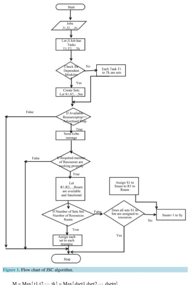
The followingFigure 1, shows the flow chart of Job Scheduling Using Coupling Algorithm. The Pseudocode of Job Scheduling Using Coupling is given inAppendix A.
5. Simulation Design
Grid Simulator (Gridsim) is used for simulation. It is a tool which is used to simulate the Grid Computing Envi-ronment. This simulation contains entities for users, resources, information service, etc. Jobs are described with information like job’s execution time, necessary machine architectures. In this simulation, the dataset for job’s configuration is created randomly. Six jobs are initially used for checking the performance of the proposed algo-rithm. Then, worked out with 25 jobs and slowly increased and checked with 175 jobs. The simulation experi-ments are done 8 times and in each experiment the scheduling algorithms FCFS, MET, LTF and proposed JSC algorithm is worked out on the specific number of jobs by using 4 to 8 matching resources. The Turn Around time is calculated in every simulation experiment for different scheduling algorithms. For implementing and evaluating proposed algorithm, random number of modules are generated for each job and they are grouped in the form of sets. Each set holds the interdependent modules. The results and performance is evaluated using the performance metrics mentioned in Section 5.1.
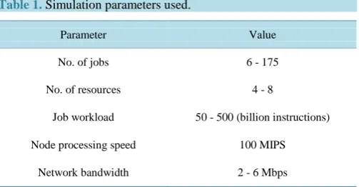
The Simulation is performed using the simulation parameters mentioned inTable 1.
5.1. Performance Metrics
Turn Around Time: Let the total number of jobs be N and the completion time of job ji is ci and the job arrival time is ai. The Total Turn Around Time is defined by the following equation
(
)
1 1 TAT
N
i
ci ai N =
=
∑
− (2)Makespan: It is defined as the time spent from the beginning of the first task to the end of the last task in the schedule. The assumptions made are resources are available continuously and jobs are ready to be scheduled. The Makespan is given as
{
}
M=Max C1, C2,C3,, Cn (3a) where Ci is the completion time of task i. Lesser the makespan means more efficient is the algorithm, i.e. less time is taken to execute the algorithm.
[image:5.595.188.440.591.722.2]For the proposed algorithm the Makespan of Job ji is
Table 1.Simulation parameters used.
Parameter Value
No. of jobs 6 - 175
No. of resources 4 - 8
Job workload 50 - 500 (billion instructions)
Node processing speed 100 MIPS
Figure 1. Flow chart of JSC algorithm.
{
}
{
}
{
} {
}
{
}
{
1 2 p}
M Max t1, t2, , tk Max dset1, dset2, , dsetp
Max C11, C12, , C1x , C21, C22, , C2y , , Ck1, Ck2, , Ckz
= =
=
(3b)
C2y are the completion times of tasks in dset2 and Ck1, Ck2, ⋅⋅⋅, Ckz are the completion times of tasks in dsetp.
5.2. An Illustrative Example
This section describes the working procedure of the proposed algorithm using 6 jobs, each with a different number of interdependent modules. Four resources are considered for illustrating this example. The following are the assumptions made while illustrating the example.
1) It is assumed that all 4 resources are working properly and available.
2) The resources advertised properties are matching with the user requested properties. 3) The interdependency among the modules for each job is given by the user.
4) The arrival time of jobs is 0 i.e. all jobs arrived at the same time.
Let 6 jobs are submitted by 6 users are {J1, J2, J3, J4, J5, J6} and the data used for each job is as follows. Let Job J1 has 3 modules/tasks, i.e., t1, t2, t3 each with execution time 2, 4, 4 secs. Tasks t1, t2 is interdepen-dent and discrete from t3. Therefore, 2 depeninterdepen-dent sets are created using the coupling phase of JSC algorithm and let, they are referred as J1S1 = {t1, t2} and J1S2 = {t3}. The total execution time of J1S1 is 6 secs and J1S2 is 4 secs. The total execution time of the job J1 is 10 secs.
Let Job J2 has 1 module/task, i.e., t1 with execution time 5 secs. Only one dependent set is created with only one task in it and let, it is referred as J2S1 = {t1} with the execution time of 5 secs.
Let Job J3 have 5 modules/tasks, i.e., t1, t2, t3, t4, t5 each with execution time 5, 2, 4, 4, 5 secs. Tasks t1, t2, t4 are interdependent and t3, t5 are interdependent. Therefore, 2 dependent sets are created using the coupling phase of JSC algorithm and let, they are referred as J3S1 = {t1, t2, t4} and J3S2 = {t3, t5}. The total execution time of each dependent set is 11 and 9 secs respectively. The total execution time of job J3 is 20 secs.
Let Job J4 have 5 modules/tasks, i.e., t1, t2, t3, t4, t5 each with execution time 4, 3, 2, 3, 5 secs. Tasks t1, t4 is interdependent and t2, t3, t5 are interdependent. Therefore, 2 dependent sets are created using the coupling phase of JSC algorithm and let, they are referred as J4S1 = {t1, t4} and J4S2 = {t2, t3, t5}. The total execution time of each dependent set is 7 and 10 secs respectively. The total execution time of job J4 is 17 secs.
Let Job J5 have 3 modules/tasks, i.e., t1, t2, t3 each with execution time 3, 2, 3 secs. Tasks t1 is discrete from other two interdependent tasks t2, t3. Therefore, 2 dependent sets are created using the coupling phase of JSC algorithm and let, they are referred as J5S1 = {t1} and J5S2 = {t2, t3}. The total execution time of each depen-dent set is 3 and 5 secs respectively. The total execution time of job J5 is 8 secs.
Let Job J6 have 6 modules/tasks, i.e., t1, t2, t3, t4, t5, t6 each with execution time 4, 3, 2, 3, 1, 2 secs. Tasks t1, t4 is interdependent, t2, t6 are interdependent and t3, t5 are interdependent. Therefore, 3 dependent sets are created using the coupling phase of JSC algorithm and let, they are referred as J6S1 = {t1, t4}, J6S2 = {t2, t6} and J6S3 = {t3, t5}. The total execution time of each dependent set is 7, 5 and 3 secs respectively. The total ex-ecution time of job J6 is 15 secs.
Using the above details the Job Scheduling algorithm third phase will allocate the resources to each dependent set of each job in parallel.
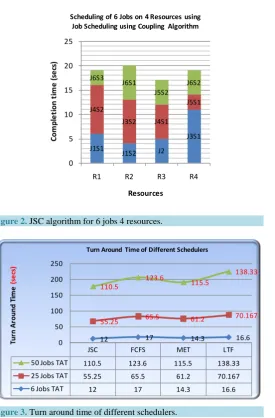
Figure 2shows the order of allocation of each dependent set of each job on 4 resources simultaneously along with the completion time of each job.
It can be observed fromFigure 2 that the completion times of Jobs {J1, J2, J3, J4, J5, J6} are {6, 5, 13, 16, 17, 20} respectively. The turn around is calculated using Equation (2) as
(
6 5 13 16 17 20)
12 secs. 6
TAT= + + + + + =
5.3. Performance
Figure 2. JSC algorithm for 6 jobs 4 resources.
Figure 3. Turn around time of different schedulers.
the queue. These algorithms executes the job sequentially and the complete job is allocated to a single resource. In these algorithms the availability of the resource and its capability of executing is not considered. The pro-posed algorithm considers nonfunctional properties such as availability and resource capability using the “echo” procedure described in Section 4. It considers only available and high performance resources and assigns the sets to the resources and sees that the sets of a job are executed simultaneously or in a parallel manner. With this approach, each job’s makespan is reduced, thereby reducing the execution time and decreasing the total turn-around time. The performance of the proposed algorithm is observed better than the existing algorithm such as FCS, MET and LTF scheduling algorithms. The total Turn Around Time of proposed algorithm is observed lesser than other algorithms considered for comparison.
InFigure 3, the three curves are the results of performing the simulation using 6, 25 and 50 jobs. Each curve shows the Turn Around Times of JSC, FCFS, MET and LTF.
It is observed in Figure 3 that the Turn Around Time of LTF and FCFS increases with an increase in the number of jobs. When MET and JSC are compared, the Turn Around time decreases with the increase in the number of jobs, but JSC’s Turn Around Time is considerably lesser than MET Turn Around Time.
6. Conclusion
In this paper, job scheduling using coupling algorithm is proposed in which the job is scheduled parallel on the J1S1 J1S2 J2
J3S1 J4S2 J3S2 J4S1 J5S1 J6S3 J6S1 J5S2 J6S2 0 5 10 15 20 25
R1 R2 R3 R4
Co m ple tio n tim e ( se cs ) Resources
Scheduling of 6 Jobs on 4 Resources using Job Scheduling using Coupling Algorithm
JSC FCFS MET LTF
50 Jobs TAT 110.5 123.6 115.5 138.33 25 Jobs TAT 55.25 65.5 61.2 70.167
6 Jobs TAT 12 17 14.3 16.6
12 17 14.3 16.6
55.25 65.5 61.2 70.167
110.5 123.6 115.5
138.33 0 50 100 150 200 250 Tu rn A ro un d T im e (se cs)
resources by considering the groups of dependent tasks. Each dependent set will have set of dependent modules/ tasks. Each dependent set of a job is scheduled on different resources rather than on a single resource to avoid sequential execution. The simulation is done on GridSim, and the make-span time and total turn around time of the proposed algorithm (JSC) are compared with FCFS, MET and LTF algorithms. The JSC algorithm will se-lect only the resources which are available and performing well, i.e. the non functional properties of a resource are considered in selecting the resources from the matching set before proceeding with the actual allocation of a dependent set of a job on a resource. As JSC algorithm is executing the job’s tasks simultaneously in a parallel manner on different matching resources, the turn around time and make-span time are observed to be reduced considerably when compared to the FCFS, MET, and LTF. The coupling concept mentioned in Section 3 meas-ures whether a module is dependent on another module or not. But, it will not give the information about the module details on which the current module is dependent. Therefore, in the proposed algorithm the dependency sets are created using the user given details about the modules or tasks of a job, i.e., the JSC algorithm depends on the user given information about the details of the interdependent modules or tasks. If this dependency check and identification of dependent tasks are done by the Grid Resource Manager rather than depending on the user’s input, the user’s burden will be reduced. Therefore, identification of the interdependent tasks after the job is submitted to grid remains the future work of this proposed work.
References
[1] Kesselman, C., Foster, I. and Steven, T. (2001) The Anatomy of the Grid-Enabling Scalable Virtual Organizations. The International Journal of Super Computer Application, 15, 200-222. http://dx.doi.org/10.1177/109434200101500302
[2] Andrew, R. and Krzysztof, P. (2004) Grid Computing: The Current State and Future Trends (in General). University of Canterbury, Christchurch, TR-CoSc 01/04.
[3] Paolucii, M., Kawamura, T., Payne, T. and Sycara, K. (2002) Semantic Matching of Web Service Capabilities. Pro-ceedings of 1st International Semantic Web Conference (ISWC2002), Berlin.
[4] Zhang, Z.P., Wen, L.J. and Wang, Z.P. (2013) LoBa-Min-Min-SPA: Grid Resources Scheduling Algorithm Based on Load Balance Using SPA. The Open Automation and Control Systems Journal, 5, 87-95.
http://dx.doi.org/10.2174/1874444301305010087
[5] Anitha, A. (2015) Trust Management in Grid-Trust Assessment and Trust Degree Calculation of a Resource—A Novel Approach. Journal of Computers and Communications, Scientific Research Publications, 3, 34-41.
http://dx.doi.org/10.4236/jcc.2015.36005
[6] Ahmed, I., Kwok, Y.K., Wu, M.Y. and Li, K. (2004) Experimental Performance Evaluation of Job Scheduling and Processor Allocation Algorithms for Grid Computing on Metacomputers. Proceedings of the 18th International Sym-posium Parallel Distributed Processing, IEEE Xplore Press, 170-177.
[7] Daulamis, N.D., Daulamis, A.D., Varvarigos, E.A. and Varvarigou, T.A. (2007) Fair Scheduling Algorithms in Grid. IEEE Transactions on Parallel Distributed System, 18, 1630-1648. http://dx.doi.org/10.1109/TPDS.2007.1053
[8] Yu, X.P. and Yu, X.G. (2009) A New Grid Computation-Based Min-Min Algorithm. 6th International Conference on Fuzzy Systems and Knowledge Discovery, Tianjin, 14-16 August 2009, 43-45. http://dx.doi.org/10.1109/fskd.2009.81
[9] Ni, L.N., Zhang, J.Q., Yan, C.G. and Jiang, C.J. (2005) A Heuristic Algorithm for Task Scheduling Based on Mean Load. 1st International Conference on Semantics, Knowledge and Grid (SKG’05), Beijing, 27-29 November 2005.
http://dx.doi.org/10.1109/skg.2005.13
[10] Kamalam, G.K. and Muralibhaskaran, V. (2010) A New Heuristic Approach: Min-Mean Algorithm for Scheduling Metatasks on Heterogenous Computing Systems. International Journal of Computer Science and Network Security, 10. [11] Menasce, D., Saha, D., Porto, S.C.D., Almeida, V.A.F. and Tripathi, S.K. (1995) Static and Dynamic Processor
Sche-duling Disciplines in Heterogenous Parallel Architectures. Journal of Parallel and Distributed Computing, 28, 1-18.
http://dx.doi.org/10.1006/jpdc.1995.1085
[12] Ramaparvathy, L. (2014) A New-Threshold Based Job Scheduling for Grid System. Journal of Computer Science, Science Publications, 10, 1069-1076. http://dx.doi.org/10.3844/jcssp.2014.1069.1076
[13] Madhuri, B. and Pradhan, S.N. (2011) NGSched—An Efficient Scheduling Algorithm Handling Interactive Jobs in Grid Environment. International Journal of Grid and Distributed Computing, 4, 1.
[14] Ajith, A., Rajkumar, B. and Baikunth, N. (2000) Nature’s Heuristic for Scheduling Jobs on Computational Grids. Pro-ceedings of 8th IEEE International Conference on Advanced Computing and Communications (ADCOM2000).
http://dx.doi.org/10.5121/ijgca.2012.3405
[16] Prajapathi, H.B. and Vipul, A.S. (2014) Scheduling in Grid Computing Environment. 4th International Conference on Advanced Computing & Communication Technologies (ACCT),Rohtak, 8-9 February 2014,315-324.
http://dx.doi.org/10.1109/ACCT.2014.32
[17] Armstrong, R., Hensegen, D. and Kidd, T. (1998) The Relative Performance of Various Mapping Algorithms Is Inde-pendent of Sizable Variances in Run-Time Productions. 7th IEEE Heterogenous Computing Workshop (HCW’98), Or-lando, 30 March 1998,79-87. http://dx.doi.org/10.1109/HCW.1998.666547
[18] Freund, R.F. and Siegel, H.J. (1993) Heterogenous Processing. IEEE Computer, 26, 13-17.
[19] Massimiliano, C. and Stefano, G. (2008) Resource Allocation in Grid Computing. WSEAS Transactions on Computer Research, 3.
[20] Jefferson, O.A., Mary, J.H. and Priyadarshan, K. (1996) A Software Metric System for Module Coupling. Journal of Systems & Software, 20, 295-308.
[21] Allen, E.B. and Khoshgoftaar, T.M. (2001) Measuring Coupling and Cohesion of Software Modules: An Information Theory Approach. Proceedings of 7th International Conference on Software Metric Symposium, London, 4-6 April 2001, 124-134. http://dx.doi.org/10.1109/METRIC.2001.915521
Appendix A
PseudocodeFor i = 1 to n Begin
S[]=CoupledSets(Ji)
R[]=CheckAvailable_Res(parameters); Rnum=R.length;
If S.length <= Rnum For j = 1 to m Begin
Assign(S[j],Rj) End For
Else
For j = 1 to m Begin
Assign(S[j],Rj) If j==Rnum Rnum=1 End For End If End For
Pseudocode for CheckAvailable_Res procedure
CheckAvailable_Res(parameters user_requested_parameters[]) Begin
For each registered resource Ri Begin
If match(user_requested_parameters,resource_advertised_parameters of Ri)==1) Begin
ack=send echo “hello” to resource Ri If(ack>=1and ack.time<=threshold_set_time) Begin
//Select resource and consider it as available and working properly. Add to the selected resources Add(R[ ], Ri)
End if End if End for Return R
End CheckAvailable_Res
The CheckAvailable_Res procedure sends an echo message “hello” to all registered resources. If the resource is working properly and it is available, it will send the acknowledgement (ack). If acknowledgement is received within the threshold time, which is already set, then the resource is added to the set of available resources array R [].
Pseudocode for CoupledSets(j)
CoupledSets(J) Begin
//Identify the tasks which are interdependent using user given information about the interdependency among modules
//Group them into a set, referred here as “dependent set” and add it to S []. End for