Numerical Analysis of Reliability and Availability of the Web based Software System

Numerical Analysis of Reliability and Availability of the

Web based Software System

Neeraj Kumar Sharma Raj kumar Bhagat Arun Prakash Agrawal

Amity University, Noida University of Delhi, Delhi Amity University, Noida

ABSTRACT

Today is the world of computers’ tasks where least human interventions are required and the software behave like the brain for computers. A small error in the software sub-system can cause a failure in the complete system that leads to disastrous failures which differ in their impact depending on the operations of an organization. Therefore, the analysis of software systems for their reliability and availability is of great significance. Reliability & Availability are the two most important measures for evaluating the quality of the software system and represents user-oriented view of software quality. Now a days Web based software system are the most famous one with the dawn in internet technology. Presently almost every organization is using this software system. This paper describes the numerical analysis of reliability & availability of web based software system based on architecture.

Keywords

Reliability and availability analysis, Software architecture, Software component, Markov process, software quality

1. INTRODUCTION

Software systems are increasingly entering consumers’ everyday life. These software systems are a part of almost all the computerized products developed and used by organizations as well as the consumers. Due to the uncertainties associated with parameters like software failure and repair rates, which either cannot be accurately measured in limited time frames through testing, or may vary on different customer sites. Reliability and availability analysis must be able to accommodate the uncertainties and produce meaningful results. Reliability is defined here as the probability of the failure-free operation of a software system for a specified period of time in a specified environment [1].

Availability is used to indicate the probability of a system or equipment being in operating condition at any time t, given that it was in operating condition at t = 0. Reliability and availability are often defined as attributes of dependability, which is the ability to deliver service that can justifiably be trusted [2].With the dawn of internet technology, today web services become the most powerful tool for information sharing& transactions. Here we are analyzing the architecture-based reliability and availability of the Web architecture-based software system by using Markov chain process. Section 2 describes the web architecture and its component. As well as we explain in brief the system description, notations and certain assumptions of the present work. In section 3the mathematical model for the web based software system is derived on the basis of Markov model. After that formulation of Chapman-Kolmogorov differential equation is done for determining the reliability and availability of the web-based software system. The behavior analysis of the system is carried out in section 4 for various combinations of repair and failure rates of the sub systems. The conclusion based on the numerical analysis is finally presented in section 5.

2. OVERVIEW OF WEB BASED

SOFTWARE SYSTEM

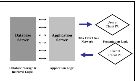
A web-based software system is an application that uses the internet infrastructure and web technologies to deliver their functionality and can be accessed through the web browser [3]. The software and database reside on a central server rather than being installed on the desktop system and is accessed over a network. Two-tier and three-tier architecture are two commonly used approaches for web based software systems. We are taking three-tier architecture of the web system for analysis.

2.1 Description of Three-Tier Architecture

Most applications deployed on the web, implement a three-tier architecture comprising of a database three-tier at the bottom, the application tier in the middle and the client tier on top. Three-tier architecture is the most common approach used for web based software systems. Three-tier architecture consists of the following three layers (tiers)

(i) Client-tier: This tier is responsible for the presentation of data, receiving user events and controlling the user interface. The actual business logic is hidden from client tier. (ii) Application-server-tier: This tier protects the data from direct access by the clients and is not present in two-tier architecture. An application server is a software framework dedicated to the efficient execution of procedures for supporting the construction of applications. It processes the inputs it receives from the clients and interacts with the database. This tier consists of the web server, web scripting language and the scripting language engine.

[image:2.595.46.518.90.372.2]

Figure 2.1

2.2 Components of the Web-Based Software

System

The web-based software system consists of four main components namely

(i) Application servers (AP): Four application servers namely A1, A2, A3 and A4 are considered here, which are present in the system. The system works in full capacity if all the APs are in working state. As soon as failure occurs in one of the APs the system goes to the reduced state. The user should get the results in some desired amount of time after which the failure in the system is assumed. If the failure occurs in the three or more APs, we assume that the system fails as the user gets the web pages after a long time of wait. So, at least three APs must be running to keep the system working. The system fails if three out of four APs fail.

(ii) Database servers (DB): The two database servers, namely, D1 and D2 are considered here, used for processing various database queries of the system. Both the DBs should be working to get the result of the query in minimum possible time. If one of the DBs fails the performance of the system goes down and the system is said to be working in reduced state. If both DBs fail the system goes to the failed state. (iii) Routers (RT): The two routers, namely, R1 and R2 are considered here, used for transferring data packets to the destinations based on their addresses. If there is a failure in one of the RTs the availability of the system goes

down and it works in the reduced state. If both the RTs fail the system fails.

(iv) Backbone Networks: we are considering that there is no failure in the backbone networks.

3. MATHEMATICAL FORMULATION

OF WEB-BASED SOFTWARE

SYSTEM

In this section we are developing the state based Markov model for web based software system on the basis of components of the web system described in section 2.2

3.1 Description of States

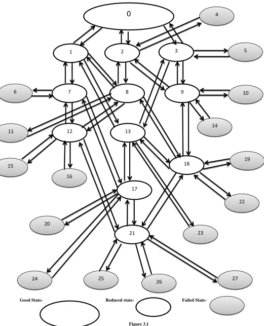
The description of states shown in fig. 3.1 is presented in the quadruple form:

(State, number of application servers working, number of database servers working, number of routers working).

We are considering that the system remains in either of three states i.e. Good state, Reduced state or Failed state, depending on the number of database server, application server and routers working. We start with the state 0 when all the APs,

DBs & RTs are working. The state is represented as (0,4,2,2). If we take a general combination of DBs, APs & RTs then total number of possible states would be 45 for Markov model but all of these states are not valid. Out of 45 only 28 states are valid since failure state after failed state is not considered for the model. The state descriptions of other states are shown below

Data Flow Over

Network Presentation Logic

Database Storage & Application Logic

Retrieval Logic

Database

Server

Application

Server

User at

Client PC

[image:3.595.15.537.110.754.2]

Good State- Reduced state- Failed State-

Figure 3.1

1

0

2

3

7

8

9

18

12

13

16

22

17

20

23

21

4

10

14

19

6

11

15

24

25

27

26

(1,3,2,2), (2,4,1,2), (3,4,2,1), (4,4,0,2), (5,4,2,0), (6,1,2,2), (7,2,2,2), (8,3,1,2), (9,4,1,1), (10,4,0,1), (11,3,0,2), (12,2,1,2), (13,3,2,1), (14,4,1,0), (15,2,0,2), (16,1,1,2), (17,2,2,1), (18,3,1,1), (19,3,0,1), (20,2,2,0), (21,2,1,1), (22,3,1,0), (23,3,2,0), (24,1,2,1), (25,1,1,1), (26,2,1,0) and (27,2,0,1).

3.2 Description of Edges

The description about all the edges shown in fig. 3.1 is presented in the following triplet form:

(source node, destination node, weight of the edge)

The weight of the edge is either repair rate or failure rate of a subsystem. Thus the triplet (0,1,4X1)represents that state 0 is

transferred to state 1 with failure rate 4X1.On the basis of the transition diagram, descriptions of other connectors are presented in the following triplet:

(0,2,2X2), (0,3,2X3), (1,0,Y1), (1,7,3X1), (1,8,2X2),

(1,13,2X3), (2,0,Y2), (2,4,X2), (2,8,4X1), (2,9,2X3),

(3,0,Y3), (3,5,X3), (3,9,2X2), (3,13,4X1), (4,2,Y2),

(5,3,Y3), (6,7,Y1), (7,1,Y1), (7,6,2X1),

(7,12,2X2),(7,17,2X3),(8,1,Y2), (8,2,Y1), (8,11,X2),

(8,12,3X1), (8,18,2X3), (9,2,Y3), (9, 3,Y2), (9,10,X2),

(9,14,X3), (9,18,4X1), (10,9,Y2), (11,8,Y2), (12,7,Y2),

(12,8,Y1), (12,15,X2), (12,16,2X1), (12,21,2X3),

(13,1,Y3), (13,3,Y1),

(13,17,X1),(13,18,2X2),(13,23,X3),(14,9,Y3),

(15,12,Y2), (16,12,Y1), (17,7,Y3), (17,13,Y1),

(17,20,X3), (17,21,2X2) , (17,24,2X1), (18,8,Y3),

(18,9,Y1), (18,13,Y2), (18,19,X2), (18,21,3X1),

(18,22,X3), (19,18,Y2), (20,17,Y3), (21,12,Y3),

(21,17,Y2), (21,18,Y1), (21,25,2X1), (21,26,X3),

(21,27,X2), (22,18,Y3), (23,13,Y3), (24,17,Y1),

(25,21,Y1), (26,21,Y3) and (27,21,Y2).

3.3 Notations

(t): Probability that the system is in state i at time t (i = 0, 1,…, 27).

(t): Derivative of Pi(t) with respect to time t (i = 0,

1,…, 27).

X1: Failure rate of application server caused by fault

in software.

Y1: Software repair rate in application server

X2: Failure rate of database server caused by fault in

software.

Y2: Software repair rate in database server.

X3: Failure rate of routers caused by fault in router

software.

Y3: Software repair rate in router.

3.4 Transient State for Reliability Analysis

With probability considerations of various states, in transition diagram shown in fig. 3.1, the following system of linear differential equations is obtained at time t using mnemonic rule. The differential equation of state 0 is written as

P0(t)(t+Δt) = [1-(4X1+2X2+2X3)]P0(t)Δt=Y1P1(t)Δt+

Y2P2(t)Δt+Y3P3(t)Δt

Dividing both sides by Δt and taking limit as Δt→0, we get

P0ꞌ(t)+(4X1+2X2+2X3)P0(t)= Y1P1(t)+Y2P2(t)+Y3P(t)

………...(3.1)

Similarly, differential equations for the other states can be written as

P1ꞌ(t)+(3X1+Y1+2X2+2X3)P1(t)=4X1P0(t)+Y1P7(t)

+Y2P8(t)+Y3P13(t)………(3.2)

P2ꞌ(t)+(Y2+4X1+X2+2X3)P2(t)=2X2P0(t)+Y1P8(t)

+Y3P9(t)+Y2P4(t)……….(3.3)

P3ꞌ(t)+(Y3+4X1+2X2+X3)P3(t)=2X3P0(t)+Y3P5(t)

+Y1P13(t)+Y2P9(t)………..……….(3.4)

P4ꞌ(t)+Y2P4(t)=X2P2(t)………(3.5)

P5ꞌ(t)+Y3P5(t)=X3P3(t)………..(3.6)

P6ꞌ(t)+Y1P6(t)=2X1P7(t)………(3.7)

P7ꞌ(t)+(2X1+2X2+Y1)P7(t)=3X1P1(t)+Y1P6(t)

+Y2P12(t)+Y3P17(t)………...(3.8)

P8ꞌ(t)+(Y1+Y2+3X1+X2+2X3)P8(t)=2X2P1(t)

+4X1P2(t)+Y1P12(t)+Y2P11(t)+Y3P18(t)………….(3.9)

P9ꞌ(t)+(Y3+Y2+4X1+X2+X3)P9(t)=2X3P2(t)+2X2P3(t)+Y

2P10(t)+Y3P14(t)+Y1P18(t)………...(3.10)

P10ꞌ(t)+Y2P10(t)=X2P9(t)……….……….(3.11)

P11ꞌ(t)+Y2P11(t)=X2P8(t)………..(3.12)

P12ꞌ(t)+(Y1+Y2+X2+2X1+2X3)P12(t)=3X1P8(t)

+2X2P7(t)+Y2P15(t)+Y1P16(t)+Y3P21(t)…………(3.13)

P13ꞌ(t)+(Y3+Y1+2X2+3X1+X3)P13(t)=2X3P1(t)

+4X1P3(t)+Y2P18(t)+Y1P17(t)+Y3P23(t)…………(3.14)

P14ꞌ(t)+Y3P14(t)=X3P9(t)………..(3.15)

P15ꞌ(t)+Y2P15(t)=X2P12(t)………(3.16)

P16ꞌ(t)+Y1P16(t)=2X1P12(t)………..(3.17)

P17ꞌ(t)+(Y1+Y3+X3+2X1+2X2)P17(t)=2X3P7(t)

+3X1P13(t)+Y2P21(t)+Y3P20(t)+Y1P24(t)………..(3.18)

P18ꞌ(t)+(Y1+Y2+Y3+3X1+X2+X3)P18(t)=2X2P13(t)

+2X3P8(t)+4X1P9(t)+Y2P19(t)+Y1P21(t)+Y3P22(t)………

………(3.19)

P19ꞌ(t)+Y2P19(t)=X2P18(t)………(3.20)

P20ꞌ(t)+Y3P20(t)=X3P17(t)………(3.21)

P21ꞌ(t)+(Y1+Y2+Y3+2X1+X2+X3)P21(t)=3X1P18(t)

+2X2P17(t)+2X3P12(t)+Y1P25(t)+Y2P27(t)+Y3P26(t)……

P22ꞌ(t)+Y3P22(t)=X3P18(t)………(3.23)

P23ꞌ(t)+Y3P23(t)=X3P13(t)………(3.24)

P24ꞌ(t)+Y1P24(t)=2X1P17(t)………..(3.25)

P25ꞌ(t)+Y1P25(t)=2X1P21(t)………..(3.26)

P26ꞌ(t)+Y3P26(t)=X3P21(t)…………..……….….(3.27)

P27ꞌ(t)+Y2P27(t)=X2P21(t)……….………...(3.28)

With initial condition P0(0)



and Pj(0)=0

for ( j 1,2,…...,27)………(3.29)

The initial condition is based on the assumption that all the components are in the working state in the beginning. The system of linear differential equations (3.1-3.28) is called Chapman-Kolmogorov differential equation. Once the system of differential equations (3.1-3.28) together with initial condition (3.29) has been solved, the reliability R(t)of the system can be calculated using the following relation

R(t)= P0(t)

+

P1(t)+ P2(t)+ P3(t)+ P7(t)+ P8(t)+ P9(t)+

P12(t)+P13(t)+P17(t)+P18(t)+P21(t)………(3.30) Mean time between failures (MTBF) has been calculated using

MTBF= ………..……...(3.31)

3.5 Steady State for Availability Analysis

System analysts are always interested in the long run availability. For this, we need to find the steady state probability of the system which can be obtained by imposing the condition as

0, as t .

Thus, the system of linear differential equations (3.1-3.28) now reduces to the following system of linear equations:

(4X1+2X2+2X3)P0(t)=Y1P1(t)+Y2P2(t)+Y3P(t)... ...(3.32)

(3X1+Y1+2X2+2X3)P1(t)=4X1P0(t)+Y1P7(t)+Y2P8(t)+Y3

P13(t)………..(3.33)

(Y2+4X1+X2+2X3)P2(t)=2X2P0(t)+Y1P8(t)+Y3P9(t)

+Y2P4(t)……….(3.34)

(Y3+4X1+2X2+X3)P3(t)=2X3P0(t)+Y3P5(t)+Y1P13(t)

+Y2P9(t)………..………(3.35)

Y2P4(t)=X2P2(t)……….………..(3.36)

Y3P5(t)=X3P3(t)……….………..(3.37)

Y1P6(t)=2X1P7(t)……….………(3.38)

(2X1+2X2+Y1)P7(t)=3X1P1(t)+Y1P6(t)+Y2P12(t)

+Y3P17(t)………...(3.39)

(Y1+Y2+3X1+X2+2X3)P8(t)=2X2P1(t)+4X1P2(t)

+Y1P12(t)+Y2P11(t)+Y3P18(t)……….(3.40)

(Y3+Y2+4X1+X2+X3)P9(t)=2X3P2(t)+2X2P3(t)

+Y2P10(t)+Y3P14(t)+Y1P18(t)………...(3.41)

Y2P10(t)=X2P9(t)……….……….(3.42)

Y2P11(t)=X2P8(t)………..(3.43)

(Y1+Y2+X2+2X1+2X3)P12(t)=3X1P8(t)+2X2P7(t)

+Y2P15(t)+Y1P16(t)+Y3P21(t)……….(3.44)

(Y3+Y1+2X2+3X1+X3)P13(t)=2X3P1(t)+4X1P3(t)

+Y2P18(t)+Y1P17(t)+Y3P23(t)………(3.45)

Y3P14(t)=X3P9(t)………..(3.46)

Y2P15(t)=X2P12(t)………(3.47)

Y1P16(t)=2X1P12(t)………..(3.48)

(Y1+Y3+X3+2X1+2X2)P17(t)=2X3P7(t)+3X1P13(t)

+Y2P21(t)+Y3P20(t)+Y1P24(t)………...…(3.49)

(Y1+Y2+Y3+3X1+X2+X3)P18(t)=2X2P13(t)+2X3P8(t)

+4X1P9(t)+Y2P19(t)+Y1P21(t)+Y3P22(t)……….(3.50)

Y2P19(t)=X2P18(t)………(3.51)

Y3P20(t)=X3P17(t)………(3.52)

(Y1+Y2+Y3+2X1+X2+X3)P21(t)=3X1P18(t)+2X2P17(t)

+2X3P12(t)+Y1P25(t)+Y2P27(t)+Y3P26(t)………..(3.53)

Y3P22(t)=X3P18(t)………(3.54)

Y3P23(t)=X3P13(t)………(3.55)

Y1P24(t)=2X1P17(t)………..(3.56)

Y1P25(t)=2X1P21(t)………..(3.57)

Y3P26(t)=X3P21(t)………..……….….(3.58)

Y2P27(t)=X2P21(t)……….………...(3.59)

The system of linear equations (3.32-3.59) together with the normalizing condition



can be solved to find the unknown Pi(t) (i 1,...,27). Once

these unknowns are known, the system availability A(



) can be calculated using the following relation

A

(



)



P0

+

P1+ P2+ P3+ P7+ P8+ P9+ P12+ P13+P17+

4. BEHAVIOUR ANALYSIS OF

WEB-BASED SYSTEM

4.1 Transient State

In this section we have studied the effect of software failure and repair rates of application server, database server and routers on the reliability of the system following the approach of Gupta et al. [13]. The system of differential equation (3.1-3.28) together with initial condition (3.29) has been solved numerically using Runge-Kutta fourth order method, assuming step size h=0.005 as one hour and finally computed reliability of the system using relation (3.30) for various combination of failure and repair rates of the subsystems. The data for failure and repair rates of the various subsystems is the actual data taken in the units of per hour. The MTBF is finally computed from the equation (3.31) using Simpson rule.

4.1.1 Variation in the reliability of the system

with the change in software failure rates of

Application server

The reliability of the system has been calculated for various values of software failure rates (X1=0.02, 0.03, 0.04, 0.05,

[image:6.595.311.546.189.313.2]

0.06) of the Application server and keeping other parameters: X2=0.03, X3=0.01, Y1=1, Y2=3, Y3=2 fixed. We have also computed MTBF of the system and the results are presented in Table 4.1.

Table 4.1

Time( hrs.)

X1=0.02 X1=0.03 X1=0.04 X1=0.05 X1=0.06

50 0.99971 0.99953 0.99931 0.99891 0.99835 100 0.99961 0.99931 0.99873 0.99793 0.99661 150 0.99959 0.99921 0.99852 0.99749 0.99605 200 0.99958 0.99919 0.99848 0.99735 0.99582 250 0.99958 0.99918 0.99845 0.99733 0.99571 300 0.99958 0.99918 0.99845 0.99732 0.99573 350 0.99958 0.99918 0.99845 0.99733 0.99572 400 0.99958 0.99918 0.99846 0.99732 0.99574 450 0.99958 0.99918 0.99846 0.99733 0.99574 500 0.99958 0.99918 0.99846 0.99733 0.99574

MTBF 433.155 432.996 432.711 432.250 431.613

4.1.2 Variation in the reliability of the system

with the change in software failure rates of

database server

The reliability of the system has been calculated for various values of software failure rates (X2=0.01, 0.02, 0.03, 0.04,

0.05) of the database server and keeping other parameters:

[image:6.595.49.285.379.498.2]

X1=0.04, X3=0.01Y1=1, Y2=3, Y3=2fixed. We have also computed MTBF of the system and the results are presented in Table 4.2.

Table 4.2

Time (hrs.)

X2=0.01 X2=0.02 X2=0.03 X2=0.04 X2=0.05

50 0.99947 0.99944 0.99932 0.99916 0.99896 100 0.99893 0.99885 0.99876 0.99862 0.99843 150 0.99871 0.99866 0.99855 0.99838 0.99821 200 0.99866 0.99858 0.99847 0.99832 0.99813 250 0.99863 0.99858 0.99846 0.99830 0.99812 300 0.99863 0.99856 0.99845 0.99830 0.99811 350 0.99863 0.99856 0.99845 0.99831 0.99811 400 0.99863 0.99856 0.99846 0.99831 0.99811 450 0.99863 0.99856 0.99846 0.99831 0.99811 500 0.99863 0.99856 0.99846 0.99831 0.99811

MTBF 432.782 432.752 432.704 432.640 432.558

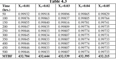
4.1.3 Variation in the reliability of the system

with the change in software failure rates of

routers

The reliability of the system has been calculated for various values of software failure rates (X3=0.01, 0.02, 0.03, 0.04,

0.05) of the routers and keeping other parameters: X1=0.04,

X2=0.03, Y1=1, Y2=3, Y3=2 fixed. We have also computed

MTBF of the system and the results are presented in Table 4.3.

Table 4.3

Time (hrs.)

X3=0.01 X3=0.02 X3=0.03 X3=0.04 X3=0.05

50 0.99932 0.99918 0.99896 0.99865 0.99829 100 0.99876 0.99863 0.99837 0.99805 0.99764 150 0.99855 0.99840 0.99816 0.99781 0.99741 200 0.99847 0.99835 0.99809 0.99776 0.99735 250 0.99846 0.99833 0.99807 0.99774 0.99732 300 0.99845 0.99834 0.99807 0.99775 0.99731 350 0.99845 0.99833 0.99807 0.99774 0.99733 400 0.99846 0.99833 0.99807 0.99774 0.99733 450 0.99846 0.99833 0.99807 0.99774 0.99733 500 0.99846 0.99833 0.99807 0.99774 0.99733

MTBF 432.704 432.644 432.539 432.395 432.215

4.1.4 Variation in the reliability of the system

with the change in software repair rates of

Application server

The reliability of the system has been calculated for various values of software repair rates (Y1=1, 1.1, 1.2, 1.3, 1.4) of the Application server keeping other parameters: X1=0.04,

X2=0.03, X3=0.01, Y2=3, Y3=2 fixed. We have also

[image:6.595.311.547.438.557.2]

computed MTBF of the system and the results are presented in Table 4.4.

Table 4.4

Time (hrs.)

Y1 = 1.0 Y1 = 1.1 Y1 = 1.2 Y1 = 1.3 Y1 = 1.4

50 0.99932 0.99937 0.99941 0.99945 0.99949 100 0.99876 0.99896 0.99909 0.99922 0.99931 150 0.99855 0.99881 0.99901 0.99915 0.99926 200 0.99847 0.99876 0.99897 0.99914 0.99925 250 0.99846 0.99878 0.99898 0.99913 0.99926 300 0.99845 0.99876 0.99898 0.99914 0.99926 350 0.99845 0.99876 0.99898 0.99914 0.99926 400 0.99846 0.99877 0.99898 0.99914 0.99926 450 0.99846 0.99877 0.99898 0.99914 0.99926 500 0.99846 0.99877 0.99898 0.99914 0.99926

MTBF 432.704 432.822 432.908 432.972 433.021

4.1.5 Variation in the reliability of the system

with the change in software repair rates of

database server

The reliability of the system has been calculated for various values of software repair rates (Y2=3, 3.1, 3.2, 3.3, 3.4) of the database server keeping the other parameters fixed:

X1=0.04, X2=0.03, X3=0.01, Y1=1, Y3=2. We have also computed MTBF of the system and the results are presented in Table 4.5.

Table 4.5

Time (hrs.)

Y2 = 3.0 Y2 = 3.1 Y2 = 3.2 Y2 = 3.3 Y2 = 3.4

[image:6.595.47.284.630.745.2]

450 0.99846 0.99847 0.99848 0.99849 0.99851 500 0.99846 0.99847 0.99848 0.99849 0.99851

MTBF 432.705 432.711 432.715 432.719 432.723

4.1.6 Variation in the reliability of the system

with the change in software repair rates of

routers

The reliability of the system has been calculated for various values of software repair rates (Y3=2, 2.1, 2.2, 2.3) of the

router keeping the other parameters: X1=0.04, X2=0.03,

[image:7.595.311.552.124.189.2]

X3=0.01, Y1=1, Y2=3 fixed. We have also computed MTBF of the system and the results are presented in Table 4.6.

Table 4.6

Time (hrs.)

Y3 = 2.0 Y3 = 2.1 Y3 = 2.2 Y3 = 2.3

50 0.999323 0.999326 0.999329 0.999332 100 0.998767 0.998772 0.998776 0.998779 150 0.998546 0.998551 0.998555 0.998558 200 0.998479 0.998484 0.998488 0.998491 250 0.998461 0.998466 0.998470 0.998473 300 0.998457 0.998461 0.998466 0.998469 350 0.998467 0.998462 0.998466 0.998469 400 0.998460 0.998464 0.998469 0.998472 450 0.998460 0.998465 0.998469 0.998472 500 0.998460 0.998465 0.998469 0.998472

MTBF 432.7049 432.7066 432.7082 432.7089

4.2 Steady State

In this section we have studied the effect of software failure and repair rates of application server, database server and routers on the availability of the system following the approach of Gupta et al. [13]. The system of linear equation (3.32-3.59) together with the normalizing condition



have been solved using Gauss Jacobi method. Finally, the availability of the system has been calculated using relation (3.60) for various combinations of failure and repair rates of the subsystems. The data for failure and repair rates of the various subsystems is the actual data taken in the units of per hour.

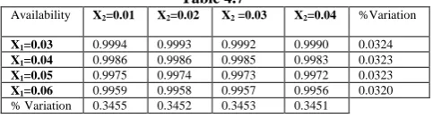
4.2.1 Sensitivity analysis of availability of

system to software failure rates of application

server and database server

The availability of the system has been calculated for various values of software failure rates of application server and database server keeping the other parameters: X3= 0.01,

Y1=1, Y2=3, Y3=2 fixed. The values of X1are taken as:

0.03, 0.04, 0.05, 0.06 and that of X2 as: 0.01, 0.02, 0.03,

[image:7.595.53.271.210.325.2]

and 0.04 and the results are presented in Table 4.7.

Table 4.7

Availability X2=0.01 X2=0.02 X2 =0.03 X2=0.04 %Variation

X1=0.03 0.9994 0.9993 0.9992 0.9990 0.0324

X1=0.04 0.9986 0.9986 0.9985 0.9983 0.0323

X1=0.05 0.9975 0.9974 0.9973 0.9972 0.0323

X1=0.06 0.9959 0.9958 0.9957 0.9956 0.0320

% Variation 0.3455 0.3452 0.3453 0.3451

4.2.2 Sensitivity analysis of availability of

system to software failure rates of application

server and router software

The availability of the system has been calculated for various values of software failure rates of application server and router software keeping the other parameters: X2=0.03,

Y1=1, Y2=3, Y3=2 fixed. The values of X1are taken as:

0.03, 0.04, 0.05, 0.06 and that of X3 as: 0.01, 0.02, 0.03, and 0.04 and the results are presented in

Table 4.8.

Table 4.8

Availability X3 =0.01 X3=0.02 X3 =0.03 X3=0.04 %Variation

X1=0.03 0.9992 0.9990 0.9988 0.99846 0.0720

X1=0.04 0.9985 0.9983 0.9981 0.99774 0.0717

X1=0.05 0.9973 0.9972 0.9969 0.99661 0.0717

X1=0.06 0.9957 0.9956 0.9954 0.99502 0.0716

% Variation 0.3453 0.3452 0.3449 0.34493

5. CONCLUDING OBSERVATIONS

[image:7.595.48.290.619.685.2]

For software systems where reliability and availability are very critical parameters, the difference in achieved and required levels of reliability and availability, by analyzing results, can help in determining the testing intensity or required manpower for the projects. The results also describe the operational performance of software system. Moreover, by analyzing the effect of failure and repair rates of various components software system for it’s the reliability and availability, we can also identify the most sensitive component of the software system. Here, it is Application server. The failure rates of this sensitive component should be minimized and the repair rates should be maximized in order to achieve the desired level of the reliability and availability of the system.

REFERENCES

[1] Reussner, R.H., Schmidt, H.W., Poernomo, I.H.: Reliability prediction for component-based software architectures. J. Systems Softw., pp.241–252, Vol. 66(3) (2003)

[2] Avizienis, A., Laprie, J.C., Randell, B.: Fundamental Concepts of Dependability. LAAS-CNRS, p. 21 (2001)

[3] Suri, P.K. and Bhushan Bharat : Reliability evaluation of web based software, International Journal of Computer Science and Network Security, pp.151- 156 , Vol. 7(9) (2007)

[4] Lyu, M. R. , Software Reliability Engineering, A Roadmap, in proceedings of international conference on Future of Software Engineering, Washington, pp.153-170 (2007)

[5] Goseva-Popstojanova, K., Trivedi, K.S.: Architecture based approach to reliability assessment of software systems. Perform. Evaluat., pp. 179-204, Vol. 45(2–3) (2001)

[6] Thomason, M.G.,Whittaker, J.A.: Rare failure-state in a Markov chain model for software reliability. In Proceedings of the 10th International Symposium on Software Reliability Engineering. IEEE, Boca Raton, (1999)

[7] Grassi, V.: Architecture-based dependability prediction for service-oriented computing. In: Proceedings of the Twin Workshops on Architecting Dependable Systems, International Conference on Software Engineering (ICSE 2004). Springer, Edinburgh, (2004)

[8] ISO/IEC, Software Engineering - Product Quality. Part 1: Quality Model (2001)

[9] Suri, P.K., Simulator for Risk assessment of software project based on performance measurement, International Journal of Computer Science and Network Security, pp. 23-30 Vol. 9(6) (2009)

[10] Taylor, R. and Vander, Hoek A.: Software Design and Architecture: The Once and Future Focus of Software Engineering, International conference on Future of Software Engineering , IEEE-CS Press, pp. 226-243 (2007)

[11] Yadav, A. and Khan R.A., Critical review on software reliability models, International Journal of recent trends in Engineering, Vol. 2(3) pp. 114-116 (2009)

[12] Immonen, A. and Niemelä, E.: Survey of reliability and availability prediction methods from the viewpoint of software architecture,Software System Model, Springer-Verlag , pp. 49–65, Vol. 7 (2007)

[13] Gupta, Pawan, Lal, A.K., Sharma, R.K. and Singh, Jai. : Numerical analysis of reliability and availability of the serial processes in butter-oil processing plant, International Journal of Quality and Reliability Management, pp. 303-316, Vol. 22(3), (2005)

[14] Taylor and Karlin: An Introduction to Stochastic Modeling, 3rd edition. Chapters 3-4.

[15] Ross: Introduction to Probability Models, 8th edition, Chapter 4.

[16] Kulkarni, V.G.: Chapter 2, Introduction to Modeling and

Analysis of Stochastic Systems, Springer Texts in Statistics, DOI 10.1007/978-1-4419-1772-0 2, Springer Science+Business Media, LLC 2011.

[17] Baresi, L., Nitto, E. and Ghezzi C.: Toward Open-World Software: Issues and challenges, IEEE Computer, pp. 36-43, Vol. 39(10) (2006)