http://dx.doi.org/10.4236/ojmsi.2015.34016
How to cite this paper: Adenomon, M.O., Michael, V.A. and Evans, O.P. (2015) A Simulation Study on the Performances of Classical Var and Sims-Zha Bayesian Var Models in the Presence of Autocorrelated Errors. Open Journal of Modelling and Simulation, 3, 146-158. http://dx.doi.org/10.4236/ojmsi.2015.34016
A Simulation Study on the Performances
of Classical Var and Sims-Zha Bayesian
Var Models in the Presence of
Autocorrelated Errors
M. O. Adenomon
*, V. A. Michael, O. P. Evans
Department of Mathematics & Statistics, The Federal Polytechnic, Bida, Nigeria
Email:
*[email protected]
,
[email protected]
,
[email protected]
Received 11 August 2015; accepted 27 September 2015; published 30 September 2015
Copyright © 2015 by authors and Scientific Research Publishing Inc.
This work is licensed under the Creative Commons Attribution International License (CC BY).
http://creativecommons.org/licenses/by/4.0/
Abstract
It is well known that a high degree of positive dependency among the errors generally leads to 1)
se-rious underestimation of standard errors for regression coefficients; 2) prediction intervals that are
excessively wide. This paper set out to study the performances of classical VAR and Sims-Zha Bayesian
VAR models in the presence of autocorrelated errors. Autocorrelation levels of (−0.99, −0.95, −0.9,
−0.85, −0.8, 0.8, 0.85, 0.9, 0.95, 0.99) were considered for short term (T = 8, 16); medium term (T = 32,
64) and long term (T = 128, 256). The results from 10,000 simulation revealed that BVAR model with
loose prior is suitable for negative autocorrelations and BVAR model with tight prior is suitable for
positive autocorrelations in the short term. While for medium term, the BVAR model with loose prior
is suitable for the autocorrelation levels considered except in few cases. Lastly, for long term, the
clas-sical VAR is suitable for all the autocorrelation levels considered except in some cases where the
BVAR models are preferred. This work therefore concludes that the performance of the classical VAR
and Sims-Zha Bayesian VAR varies in terms of the autocorrelation levels and the time series lengths.
Keywords
Simulation, Performances, Vector Autoregression (VAR), Classical VAR, Sims-Zha Prior, Bayesian
VAR (BVAR), Autocorrelated Errors
1. Introduction
Autocorrelation plays significant role in both time series and cross sectional data
[1]
. More often autocorrelation
renders the inferences and decision making about the estimated parameters invalid
[2]
. In addition, it is well
known that a high degree of positive dependency among the errors generally leads to 1) serious underestimation
of standard errors for regression coefficients; 2) prediction intervals that are excessively wide
[3]
. While
Gujara-ti,
[4]
identified the several reasons that make autocorrelation to occur. They are Inertia, Specification Bias,
Ex-cluded variables, incorrect functional form, cobweb phenomenon, lags, data transformation/manipulation, and
nonstationarity.
In the time series literature, the standard linear regression model, autocorrelation of the disturbances leads to
inefficient but still unbiased estimates of the coefficient
[5]
, while the Least squares estimation of parameters in
the general linear model may be highly inefficient in the presence of autocorrelated errors
[6]
. In the work of
Smith, Wong and Kohn,
[7]
revealed that when a regression model is fitted to time series data the errors are
likely to be autocorrelated. In a recent work of Garba
et al
.
[8]
, they observed that the autocorrelation problem
usually afflict time series data, while in a similar study carried out by Adenomon & Oyejola
[9]
, they concluded
that classical VAR model tend to forecast where there is no autocorrelation while the Bayesian VAR models
with harmonic decay forecast better for both negative and positive autocorrelation level.
This paper therefore studied the forecasting performances of the classical VAR and some versions of Sims-
Zha Bayesian VAR with quadratic decay models for bivariate time series with AR(1) error terms using Monte-
Carlo experiment.
2. Model Description
2.1. Vector Autoregression (VAR) Model
Given a set of
k
time series variables,
y
t=
[
y
it,
,
y
Kt]
′
,VAR models of the form
1 1
t t p t p t
y
=
A y
−+
+
A y
−+
u
(1)
provide a fairly general framework for the Data General Process (DGP) of the series. More precisely this model
is called a VAR process of order p or VAR(p) process. Here
u
t=
[
u
1t,
,
u
Kt]
′
is a zero mean independent
white noise process with non s
ingular time invariant covariance matrix ∑
uand the
A
iare (
k
×
k
) coefficient
ma-trices. The process is easy to use for forecasting purpose though it is not easy to determine the exact relations
between the variables represented by the VAR model in Equation (1) above
[10]
. Also, polynomial trends or
seasonal dummies can be included in the model.
The process is stable if
(
1)
det
I
K−
A z
− −
A z
p p≠
0 for
z
≤
1
(2)
In that case it generates stationary time series with time invariant means and variance covariance structure.
The basic assumptions and properties of a VAR processes is the stability condition. A VAR(
p
) processes is said
to be stable or fulfils stability condition, if all its eigenvalues have modulus less than 1
[11]
.
Therefore, to estimate the VAR model, one can write a VAR(
p
) with a concise matrix notation as
[
1]
1 1[
1]
where
,
,
,
,
,
,
tT t o T
t p
Y
BZ
U
y
Y
y
y
Z
Z
Z
Z
y
−
− −
−
=
+
=
=
=
(3)
Then the Multivariate Least Squares (MLS) for
B
yields
( )
1ˆ
B
=
ZZ
′
−Z Y
′
(4)
2.2. Bayesian Vector Autoregression with Sims-Zha Prior
sys-tem in a multivariate regression
[13]
.
Given the reduced form model
1 1
1 1 1 1 1
0 0 0 0 0
where
,
,
1, 2,
, ,
and
t t t p p t
l l t t
y
c
y
B
y
B
u
c
dA
B
A A
l
p u
ε
A
A
A
− −
− − − − −
= +
+
+
+
′
=
= −
=
=
Σ =
The matrix representation of the reduced form is given as
( 1) ( 1)
, ~
( )
0,
T m
Y
×=
T×X
mp+ mpβ
+ ×m+
T mU
×U
MVN
Σ
We can then construct a reduced form Bayesian SUR with the Sims-Zha prior as follows. The prior means for
the reduced form coefficients are that
B
1=
I
and
B
2,
,
B
p=
0
. We assume that the prior has a conditional
structure that is multivariate Normal-inverse Wishart distribution for the parameters in the model. To estimate
the coefficients for the system of the reduced form model with the following estimators
(
) (
)
(
)
(
)
1
1 1
1 1 1
ˆ
ˆ
ˆ
ˆ
X X
X Y
T
Y Y
X X
S
β
β
β
β β
β
−
− −
− − −
′
′
= Ψ +
Ψ
+
′
′
′
′
Σ =
−
+ Ψ
+ Ψ
+
where the Normal-inverse Wishart prior for the coefficients is
(
)
( )
~
N
,
and ~
IW S v
,
β
Σ
β
Ψ
Σ
This representation translates the prior proposed by Sims and Zha form from the structural model to the
re-duced form (
[13]
[14]
and
[12]
[15]
).
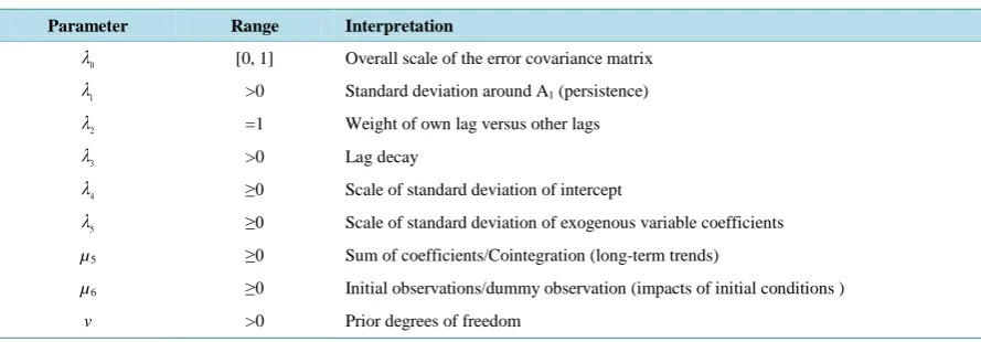
The summary of the Sims-Zha prior is given in
Table 1
.
3. Simulation Procedure
A bivariate time series data that have autocorrelated error of order 1 were simulated using the VAR (2) process
of the form:
1 1 1 1
2 2 1 2 2 2
5.0
0.5
0.2
0.3
0.7
10.0
0.2
0.5
0.1
0.3
t t t t
y
y
y
u
y
y
−y
−u
−
−
=
+
+
+
−
−
−
[image:3.595.86.531.557.712.2]Such that
u
1=
u
2=
δε
t−1+
ε
twhere
ε
t~
N
( )
0,1
. the choice here is similar to the work and illustration of
Cowpertwait,
[16]
. This work considered ten autocorrelated levels as δ = (
−0.99, −0.95, −0.9, −0.85, −0.8, 0.8,
0.85, 0.9, 0.95, 0.99) for short term (T = 8, 16); medium term (T = 32, 64) and long term (T = 128, 256). Sample
of generated data are presented in
Table 2
.
Table 1. Hyperparameters of sims-zha reference prior.
Parameter Range Interpretation
0
λ [0, 1] Overall scale of the error covariance matrix
1
λ >0 Standard deviation around A1 (persistence)
2
λ =1 Weight of own lag versus other lags
3
λ >0 Lag decay
4
λ ≥0 Scale of standard deviation of intercept
5
λ ≥0 Scale of standard deviation of exogenous variable coefficients
µ5 ≥0 Sum of coefficients/Cointegration (long-term trends)
µ6 ≥0 Initial observations/dummy observation (impacts of initial conditions )
v >0 Prior degrees of freedom
Table 2. Sample of generated data for T = 8.
Time series data for T = 8 Autocorrelated errors δ= 0.95
y1 y2
5.00505541 10.917722 0.005055408 −1.001469533
8.68460254 4.482366 −0.271733404 −1.034463062
0.82311917 9.929715 −2.226441998 −1.381950068
0.62000249 5.215348 −0.892427694 −0.108602706
−3.07110720 9.393832 0.917721826 0.942238044
0.12451823 7.026048 1.133007326 −0.131419986
−0.07930944 10.020091 −0.771095435 −0.393861135
1.90017153 7.003259 0.432758733 −0.097920078
Model Specification
The time series were generated data using a VAR model with lag 2. The choice here is to obtain a bivariate time
series with the true lag length. While the VAR and BVAR models of lag length of 2 was used for modeling and
forecasting purpose.
For the BVAR model with Sims-Zha prior, we consider the following range of values for the hyperparameters
given below and the Normal-Inverse Wishart prior was employed.
We consider two tight priors and two loose priors as follows:
(
)
(
)
0 1 3 4 5 5 6
0 1 3 4 5 5 6
0 1 3 4
The Tight priors are as follows
BVAR1
0.6, 0.1, 2, 0.1, 0.07,
5
BVAR2
0.8, 0.1, 2, 0.1, 0.07,
5
The Loose priors are as follows
BVAR3
0.6, 0.15, 2, 0
λ
λ
λ
λ
λ
µ
µ
λ
λ
λ
λ
λ
µ
µ
λ
λ
λ
λ
=
=
=
=
=
=
=
=
=
=
=
=
=
=
=
=
=
(
=
=
=
=
)
(
)
5 5 6
0 1 3 4 5 5 6
.15, 0.07,
2
BVAR4
0.8, 0.15, 2, 0.15, 0.07,
2
λ
µ
µ
λ
λ
λ
λ
λ
µ
µ
=
=
=
=
=
=
=
=
=
=
=
where
nµ
is prior degrees of freedom given as
m
+ 1 where m is the number of variables in the multiple time
se-ries data. In work
nµ
is 3 (that is two (2) time series variables plus 1(one)).
Our choice of Normal-Inverse Wishart prior for the BVAR models follow the work of Kadiyala & Karlsson,
[17]
that Normal Wishart prior tends to performed better when compared to other priors. In addition Sims and
Zha,
[12]
proposed Normal-Inverse Wishart prior because of its suitability for large systems while Breheny,
[18]
reported that the most advantage of wishart distribution is that it guaranteed to produce positive definite draws.
Our choice of the overall tightness
λ =
00.6 and 0.8
is in line with work of Brandt, Colaresi and Freeman
[19]
.
In this work we assumed that the bivariate time series follows a quadratic decay. The Quadratic Decay (QD)
model has many attractive theoretical properties that is why it is been applied to many fields of endeavour
(
[20]-[22]
).
The following are the criteria for Forecast assessments used:
1) Mean Absolute Error (
MAE
) has a formular
1n
i i j
e
MAE
n
=
=
∑
. This criterion measures deviation from the
series in absolute terms, and measures how much the forecast is biased. This measure is one of the most
com-mon ones used for analyzing the quality of different forecasts.
2) The Root Mean Square Error (
RMSE
) is given as
(
)
2n
f i i j
y
y
RMSE
n
−
=
∑
where
y
iis the time series
data and
y
fis the forecast value of
y
[23]
.
In this simulation study,
and
N N
j j
j j
RMSE
MAE
RMSE
MAE
N
N
=
∑
=
∑
where
N
= 10,000. Therefore, the model
with the minimum
RMSE
and
MAE
result as the preferred model.
4. Results and Discussion
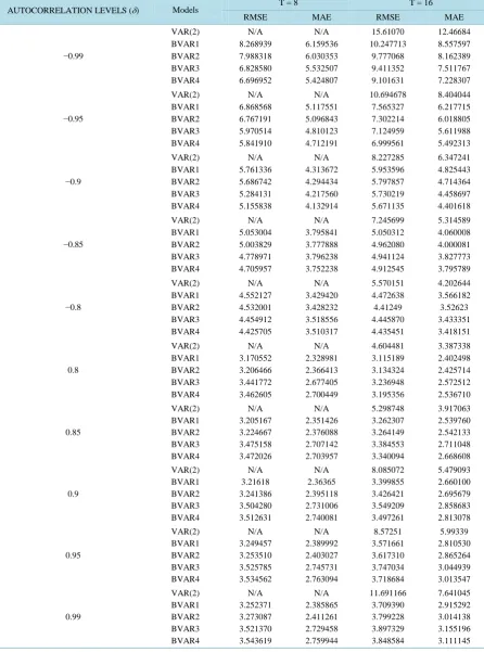
The entire simulation and analysis was carried out in R environment. The values of the RMSE and MAE for
short, medium and long terms are presented in
Tables A1-A3
respectively in
Appendix A
. While the ranks for
short, medium and long terms are presented in
Tables B1-B3
respectively in
Appendix B
. In general the values
of the RMSE and MAE increased as a result of increase in the autocorrelated levels. In addition the values of the
RMSE and MAE decreased as a result of increase in the time series lengths.
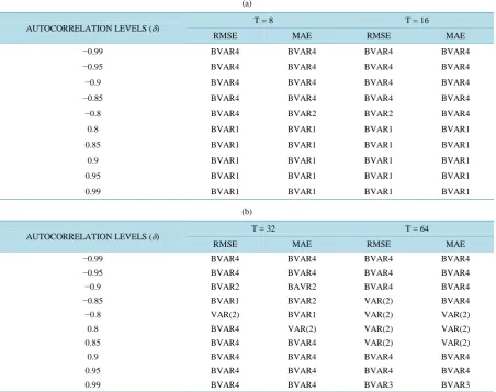
The preferred model for short, medium and long terms are presented in
Tables 3(a)-(c)
respectively.
Table 3(a)
revealed that the BVAR model with loose prior (BVAR4) is preferred for negative autocorrelation
levels except in few cases, while BVAR model with tight prior (BVAR1) is preferred for positive
autocorrela-tion levels in the short term
In
Table 3(b)
, the BVAR model with loose prior (BVAR4) is preferred for autocorrelation level of −0.99,
[image:5.595.87.540.364.721.2]−0.99 and from 0.9 to 0.99. The classical VAR (VAR(2)) is preferred for autocorrelation levels of −0.8 to 0.85
for T = 64. While in other autocorrelation levels the preferred models varies among BVAR models with tight
prior, classical VAR and BVAR model with loose prior respectively.
Table 3. (a) The preferred models for short term (T = 8, 16); (b) The preferred models for medium short (T = 32, 64); (c) The preferred models for long short (T = 128, 256).
(a)
AUTOCORRELATION LEVELS (δ) T = 8 T = 16
RMSE MAE RMSE MAE
−0.99 BVAR4 BVAR4 BVAR4 BVAR4
−0.95 BVAR4 BVAR4 BVAR4 BVAR4
−0.9 BVAR4 BVAR4 BVAR4 BVAR4
−0.85 BVAR4 BVAR4 BVAR4 BVAR4
−0.8 BVAR4 BVAR2 BVAR2 BVAR4
0.8 BVAR1 BVAR1 BVAR1 BVAR1
0.85 BVAR1 BVAR1 BVAR1 BVAR1
0.9 BVAR1 BVAR1 BVAR1 BVAR1
0.95 BVAR1 BVAR1 BVAR1 BVAR1
0.99 BVAR1 BVAR1 BVAR1 BVAR1
(b)
AUTOCORRELATION LEVELS (δ) T = 32 T = 64
RMSE MAE RMSE MAE
−0.99 BVAR4 BVAR4 BVAR4 BVAR4
−0.95 BVAR4 BVAR4 BVAR4 BVAR4
−0.9 BVAR2 BAVR2 BVAR4 BVAR4
−0.85 BVAR1 BVAR2 VAR(2) BVAR4
−0.8 VAR(2) BVAR1 VAR(2) VAR(2)
0.8 BVAR4 VAR(2) VAR(2) VAR(2)
0.85 BVAR4 BVAR4 VAR(2) VAR(2)
0.9 BVAR4 BVAR4 BVAR4 BVAR4
0.95 BVAR4 BVAR4 BVAR4 BVAR4
(c)
AUTOCORRELATION LEVELS (δ) T = 128 T = 256
RMSE MAE RMSE MAE
−0.99 BVAR3 BVAR3 BVAR2 BVAR2
−0.95 BVAR4 BVAR2 BVAR2 BVAR2
−0.9 BVAR4 BVAR4 VAR(2) VAR(2)
−0.85 VAR(2) VAR(2) VAR(2) VAR(2)
−0.8 VAR(2) VAR(2) VAR(2) VAR(2)
0.8 VAR(2) VAR(2) VAR(2) VAR(2)
0.85 VAR(2) VAR(2) VAR(2) VAR(2)
0.9 VAR(2) VAR(2) VAR(2) VAR(2)
0.95 BVAR4 BVAR4 BVAR4 BVAR4
0.99 BVAR4 BVAR4 BVAR4 BVAR2
In
Table 3(c)
, the classical VAR (VAR(2)) model is preferred for autocorrelation levels of
−0.85 to 0.9, the
BVAR model with loose prior (BVAR4) is preferred for autocorrelation levels of 0.95 and 0.99. while in other
autocorrelation levels the preferred models varies among BVAR models with loose prior, BVAR models with
tight prior and the classical VAR model respectively.
5. Conclusions and Recommendation
In conclusion, the performances of the forecasting models depend on the autocorrelation levels and the time
se-ries length.
It is therefore recommended that the autocorrelation levels and the time series length should be considered in
using an appropriate model for forecasting.
Acknowledgements
We wish to thank TETFUND Abuja-Nigeria for sponsoring this research work. Our appreciation also goes to the
Rector and the Directorate of Research, Conference and Publication of the Federal Polytechnic Bida for giving
us this opportunity to undergo this research work.
References
[1] Oloyede, I. and Yahya, W.B. (2015) Bayesian Generalized Least Squares with Autocorrelated Error. Book of Abstract
of the 34th Annual Conference of the Nigerian Mathematical Society (NMS), 23-26 June 2015.
[2] Okorie, C.E., Abubakar, U.Y and Adetutu, O.M. (2015) Analysis of Autocorrelated Data. Book of Abstract of the 34th
Annual Conference of the Nigerian Mathematical Society (NMS), 23-26 June 2015.
[3] Huitema, B.E., Mckean, J.W. and Zhao, J. (1996) The Runs Test for Autocorrelated Errors: Unacceptable Properties.
Journal of Educational & Bahaviourial Statistics, 21, 390-404. http://dx.doi.org/10.3102/10769986021004390
[4] Gujarati, D.N. (2003) Basic Econometrics. 4th Edition, The McGraw-Hill Co., New Delhi.
[5] Rao, P. and Griliches, Z. (1969) Small-Sample Properties of Several Two-Stage Regression Methods in the Context of Autocorrelated Errors. Journal of American Statistical Association, 64, 253-272.
http://dx.doi.org/10.1080/01621459.1969.10500968
[6] Berenblut, I.I. and Webb, G.I. (1973) A New Test for Autocorrelated Errors in the Linear Regression Model. Journal
of Royal Statistical Society B, 35, 33-50.
[7] Smith, M., Wong, C.-M. and Kohn, R. (1998) Additive Non-Parametric Regression with Autocorrelated Errors.
Jour-nal of Royal Statistical Society B, 60, 311-331. http://dx.doi.org/10.1111/1467-9868.00127
[8] Garba, M.K., Oyejola, B.A. and Yahya, W.B. (2013) Investigations of Certain Estimators for Modelling Panel Data Under Violations of some Basic Assumptions. Mathematical Theory and Modeling, 3, 47-53.
[9] Adenomon, M.O. and Oyejola, B.A. (2015) Forecasting Bivariate Time Series with AR(1) Error Terms. A Paper
[10] Lűtkepohl, H. and Breitung, J. (1997) Impulse Response Analysis of Vector Autoregressive Processes: System Dy-namic in Economic and Financial Models.
[11] Yang, M. (2002) Lag Length and Mean Break in Stationary VAR Models. The Econometrics Journal, 5, 374-386. http://dx.doi.org/10.1111/1368-423X.00089
[12] Sims, C.A. and Zha, T. (1998) Bayesian Methods for Dynamic Multivariate Models. International Economic Review, 39, 949-968. http://dx.doi.org/10.2307/2527347
[13] Brandt, P.T. and Freeman, J.R. (2006) Advances in Bayesian Time Series Modeling and the Study of Politics: Theory, Testing, Forecasting and Policy Analysis. Political Analysis, 14, 1-36. http://dx.doi.org/10.1093/pan/mpi035
[14] Brandt, P.T. and Freeman, J.R. (2009) Modeling Macro-Political Dynamics. Political Analysis, 17, 113-142. http://dx.doi.org/10.1093/pan/mpp001
[15] Sims, C.A. and Zha, T. (1999) Error Bands for Impulse Responses. Econometrica, 67, 1113-1155. http://dx.doi.org/10.1111/1468-0262.00071
[16] Cowpertwait, P.S.P. (2006) Introductory Time Series with R. Springer Science + Business Media, LLC., New York. [17] Kadiyala, K.R. and Karlsson, S. (1997) Numerical Methods for Estimation and Inference in Bayesian VAR Models.
Journal of Applied Econometrics, 12, 99-132.
http://dx.doi.org/10.1002/(SICI)1099-1255(199703)12:2<99::AID-JAE429>3.0.CO;2-A
[18] Breheny, P. (2013) Wishart Priors. BST 701: Bayesian Modelling in Biostatistics. http://web.as.uky.edu/statistics/users/pbreheny/701/S13/notes/3-28.pdf
[19] Brandt, P.T., Colaresi, M. and Freeman, J.R. (2008) Dynamic of Reciprocity, Accountability and Credibility. Journal
of Conflict Resolution, 52, 343-374. http://dx.doi.org/10.1177/0022002708314221
[20] Merkin, J.H. and Needman, D.J. (1990) The Development of Travelling Waves in a Simple Isothermal Chemical Sys-tem II. Cubic Autocatalysis with Quadratic and Linear Decay. Proceedings: Mathematical & Physical Sciences, 430, 315-345.
[21] Merkin, J.H. and Needman, D.J. (1991) The Development of Travelling Waves in a Simple Isothermal Chemical Sys-tem IV. Quadratic Autocatalysis with Quadratic Decay. Proceedings: Mathematical & Physical Sciences, 434, 531- 554.
[22] Worsley, K.J., Evans, A.C., Strother, S.C. and Tyler, J.L. (1991) A Linear Spatial Correlation Model with Applications to Positron Emission Tomography. Journal of the American Statistical Association, 86, 55-67.
http://dx.doi.org/10.1080/01621459.1991.10475004
[23] Caraiani, P. (2010) Forecasting Romanian GDP Using a BVAR Model. Romanian Journal of Economic Forecasting, 4, 76-87.
Appendix A
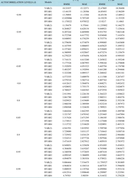
Table A1. RMSE and MAE of the Models for short term (T = 8, 16)
AUTOCORRELATION LEVELS (δ) Models T = 8 T = 16
RMSE MAE RMSE MAE
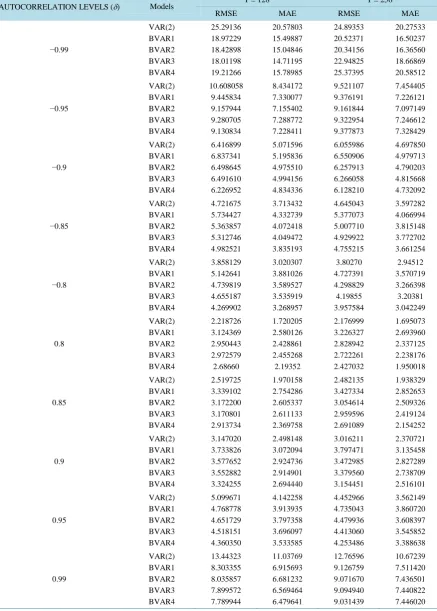
Table A2. RMSE and MAE of the models for medium term (T = 32, 64).
AUTOCORRELATION LEVELS (δ) Models T = 32 T = 64
RMSE MAE RMSE MAE
Table A3. RMSE and MAE of the models for Long term (T = 128, 256).
AUTOCORRELATION LEVELS (δ) Models T = 128 T = 256
RMSE MAE RMSE MAE
Appendix B
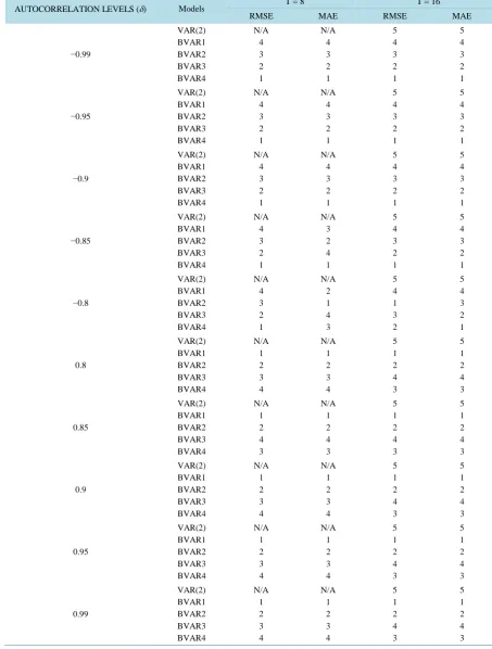
Table B1. Ranks of RMSE and MAE of the Models for short term (T = 8, 16).
AUTOCORRELATION LEVELS (δ) Models T = 8 T = 16
RMSE MAE RMSE MAE
Table B2. Rank of RMSE and MAE of the models for medium term (T = 32, 64).
AUTOCORRELATION LEVELS (δ) Models T = 32 T = 64
RMSE MAE RMSE MAE
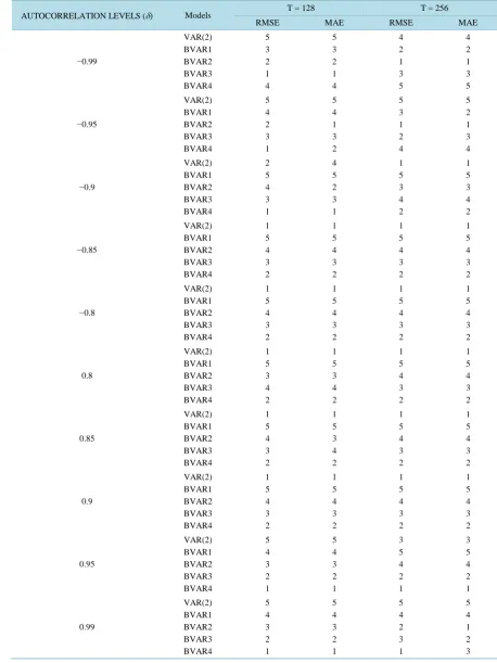
Table B3. Ranks of RMSE and MAE of the Models for Long term (T = 128, 256)
AUTOCORRELATION LEVELS (δ) Models T = 128 T = 256
RMSE MAE RMSE MAE