A Statistical Comparison of Traffic Measurements from the Moving versus Stationary Observer Methods

http://dx.doi.org/10.4236/jtts.2015.54019

A Statistical Comparison of Traffic

Measurements from the Moving versus

Stationary Observer Methods

Fadi Alhomaidat, Siamak Ardekani

Department of Civil Engineering, The University of Texas at Arlington, Arlington, USA Email: fadi.alhomaidat@uta.edu, ardekani@uta.edu

Received 8 July 2015; accepted 27 September 2015; published 30 September 2015

Copyright © 2015 by authors and Scientific Research Publishing Inc.

This work is licensed under the Creative Commons Attribution International License (CC BY). http://creativecommons.org/licenses/by/4.0/

Abstract

Data of traffic flow, speed and density are required for planning, designing, and modelling of traf-fic stream for all parts of the road system. Specialized equipments such as stationary counts are used to record volume and speed; but they are expensive, difficult to set up, and require periodic maintenance. The moving observer method was proposed in 1954 by Wardrop and Charlesworth to estimate these variables inexpensively. Basically, the observer counts the number of vehicles overtaken, the number of vehicles passed, and the number of vehicles encountered while traveling in the opposite direction. The trip time is reported for both travel directions. Additionally, the length of road segment is measured. These variables are then used in estimating speeds and vo-lumes. In a westbound direction from Interstate Highway 30 (I-30) in the DFW area, this study examined the accuracy and feasibility of this method by comparing it with stationary observer method as the standard method for such counts. The statistical tests were used to test the accuracy. Results show that this method provides accurate volume and speed estimates when compared to the stationary method for the road segment with three lanes per direction, especially when sever-al runs are taken.

Keywords

Moving Observer Method, Stationary Observer, Statistical t-Test, Traffic Measurements

1. Introduction

different methods for computing the same entity sometimes fail to confirm each other. Therefore, the observer needs to understand and study the relationship and discover any systematic correlations between the results of the two methods. Nevertheless, it is important to acquire reliable results.

The goal of this study is to determine traffic flow and speed on a three-lane interstate highway utilizing the moving observer method. The study then, compares the results from the moving observer method with the base results acquired from a stationary observer method.

Considering the significance of flow, speed, and density in traffic engineering, it is necessary to be as accurate as possible when estimating the variables. This study determines accuracy of the moving observer method by comparing the results to the estimates from the stationary observer method. Each of these two methods has a different approach and procedure for calculating traffic flow and speed. The study first used the stationary ob-server method because of its proven reliability. Then, after conducting the study using the moving obob-server me-thod, we statistically compared the results of both methods. Analysis of these results shows strong agreement between the two approaches.

2. Literature

2.1. Traffic Models Background

In general, highway traffic models can be classified as either macroscopic or microscopic. Microscopic traffic simulation focuses on individual driving behavior, such as, speeds, headways, gaps and travel times. In contrast, macroscopic traffic simulation conducts studies of average traffic characteristics, including, traffic flow, density, and space mean speed.

Data of traffic flow, speed and density are required for planning, designing, and modelling of traffic stream for all parts of the road system. However, it is difficult to measure all these variables in a single attempt. The moving observer method for traffic stream estimation has been created to facilitate the concurrent estimation of traffic stream variables [1]. This method offers an approach to obtain the complete state of the traffic stream us-ing only two observers in a movus-ing vehicle. Measurus-ing any two variables of the traffic stream will yield the third variable by using the following equation:

q=uk (1)

q: flow rate (veh/h). k: density (veh/m).

u: space mean speed (mph).

Consequently, the moving observer method is a convenient method to obtain traffic stream variables for this formula, since a speed and flow are measured and the density can be estimated. The stationary observer method for determining flow, speed, and density is quite different from the moving observer method. It focuses primari-ly on the specific point on the road section. However, the moving observer method relies on data collected by travelling along same road section. In such methods, the flow, speed, and density must be estimated by several complete travel cycles in order to increase the degree of accuracy.

2.2. Study Area

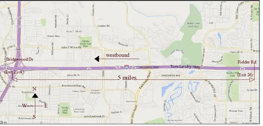
The I-30, one of the most congested urban highways in the Dallas Fort Worth (DFW) area in Texas, was selected for this study to determine traffic flow and speed using the moving observer method. Average Daily Traffic (ADT) volumes obtained from the North Central Texas Council of Government (NCTCOG) website for the westbound direction on a section from the Fielder Rd and I-30 interchange point (exit 26) to the Bridgewood Drive and I-30 interchange point (exit 21 A) reach 70,000 vehicles/day. There are three lanes in this segment and the segment length is 5.0 miles. The westbound direction was chosen to conduct the corresponding stationary observations as there were some convenient locations for video recording.

3. Methodology

3.1. Moving Observer Method

density. [1] proposed the original “moving observer method” as a method of estimating the average flow and travel time of traffic moving in one or the other direction on a freeway segment. The method was founded upon the measurements made by the moving observer in a test vehicle embedded in the traffic. The observer traveled in a test car in the direction of the stream considered with the flow while counting the number of vehicles over-taken and the number of vehicles passed. Travel is also made against the flow in the other direction, to record the number of opposing vehicles faced in the opposite direction (direction of interest) during the trip see Figure 1. In both travel directions, the trip time of the test car is recorded. Additionally, the length of the road segment is known. These measurements are then used in calculating the speed-flow relationship for the road segment in the direction of interest. Several runs are conducted to increase the accuracy.

The following information for each run is recorded by the observer in the test vehicle: 1) The number of vehicles overtaking the test vehicle.

2) The number of vehicles passing the test vehicle.

3) The number of vehicles encountered; while traveling opposite to the direction of interest.

4) The segment length and the trip time of the observer in both directions, with and against the flow traffic. [1] stated that the advantages of using the moving observer method include the following points:

1) The observer can collect the information on flow and speed simultaneously (this is valuable when seeking the relationship between these two variables).

2) The observer can measure travel time along the length of the road segment and also the flow rate and the average speed of vehicles.

3) The amount of man power and hours needed to attain a high level of accuracy is less for the moving ob-server method compared to other methods, thus making it less expensive.

4) Vehicles can be grouped and flow rates can be estimated for each group.

5) The observer can chronicle supplementary information such as the locations and causes of delays if appli-cable.

However, [2] identified some issues with the moving observer method including:

A A

X

B B

west

O

O yo

yp

L

 The observer requires a number of test runs when traffic flows are low (200 - 300 veh/hour for two lanes, one direction) to accomplish a specified level of accuracy, and this might be infeasible.

 The traffic volume that moves into the test road section changes according to the total number of intersec-tions.

 The accuracy for measuring speed and flow is very sensitive to the variations in the traffic stream along the road section at different times of the day.

3.1.1. Observations

A section of a three-lane freeway was chosen for this project. The site for the study was selected based on the following criteria:

1) Section representing the road was delineated starting from an on-ramp interchange which increases traffic flow and ending with the off-ramp interchange at the end of the segment that permits a quick turnaround for the test vehicle.

2) Section without obstacles or lanes with changed geometric features such as high-occupancy vehicle (HOV) lane was selected to provide a clear vision for the observer.

3) Section without vertical and horizontal curves to provide a clear vision for the observer in the opposite di-rection.

4) Section with high traffic flow to increase confidence in the results.

Data was collected on the westbound direction of an I-30 segment in an urban three-lane highway. The seg-ment begins from the Fielder Rd and I-30 interchange point (exit 26) and ends at the Bridgewood Drive and I-30 interchange point (exit 21 A), in the Dallas-Fort Worth (DFW) area of Texas as shown in Figure 2. Data re-quired for estimating space mean speed, flow rate, and density for moving observer method were collected on the selected road segment.

3.1.2. Procedure

The moving observer method is an approach that includes the use of a probe vehicle within a traffic stream for measuring travel time, flow rate, space mean speed, and delay in a roadway section. According to The Manual of Transportation Engineering studies [3], which describes the procedure, the observer in the survey vehicle drives at the average travel speed within the traffic stream of the designated section under evaluation. However, the observer cannot travel along the section for several miles without changing speed. In order to solve this problem, the number of vehicles passed is deducted from the number of vehicles overtaken by the observer.

Off-peak daytime periods between 11:00 am and 1:00 pm were used for the data collection on Saturday, Jan-uary 24, 2015. This period was chosen because the traffic flow in that period is generally uniform [4]. The

weather conditions were clear and dry with an average temperature of 60˚F. This weather condition was ideal in order to avoid the influence of weather factors affecting the data collection for traffic flow and speed, as men-tioned in a previous study [5].

During the study, a segment of 5.0 miles in length was used for data collection. The researcher performed six (6) test runs on this directional segment. [4] has found that six runs are adequate for reliable and unbiased esti-mates for measuring variables. In the test car, the observer held a video recording camera in order to minimize the element of human error. Therefore, real time traffic events over the entire period of the test runs were cap-tured on video. Next, the recorded traffic events were saved on computer for processing. The observer then played back the recorded traffic events in a computer to analyze events in order to obtain the required data. During the replay, the observer recorded the time it took to traverse the study segment and the number of ve-hicles encountered while traveling in the opposite direction. To calculate the hourly flow rate and the average speed for the westbound direction, the following equations were used:

p o

w a

x y y

q

t t

+ −

=

+ (2)

p o

w

y y

t t

q

−

= − (3)

nL u

t

=

∑

q = mean directional flow rate (veh/h).

x = the number of oncoming vehicles encountered while travelling in the opposite direction. yp = the test car passed vehicles.

yo = vehicles overtaking the test car (veh).

tw = the travel time to traverse the study segment with traffic (hour). ta = the travel time to traverse the study segment against traffic (hour).

u = average speed for all runs (mph). n = number of runs.

t = the mean travel times of traffic (hour). L = length of the study segment (mile).

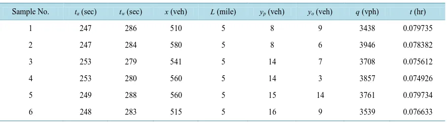
Table 1 displays the data obtained in this study.

The table shows that the flow values are 3438, 3946, 3708, 3857, 3761 and 3539 vph for the six runs, respec-tively. The mean flow value was calculated to be 3708 vph. Additionally, the mean speed was calculated using Equation (4) to be 63.2 mph. Equation (1) was then used to calculate the density, which was found to be 59.1 vpm.

The difference between the time with traffic (tw) and the time against traffic (ta) was about 30 sec for most of the runs. The time differences occurred because while travelling in the opposite direction the observer was on the left lane. Driving in the left lane helped improve the accuracy in counting the traffic in the opposite direction.

Table 1. Speed data moving observer method data.

Sample No. ta (sec) tw (sec) x (veh) L (mile) yp (veh) yo (veh) q (vph) t (hr)

1 247 286 510 5 8 9 3438 0.079735

2 247 284 580 5 8 6 3946 0.078382

3 253 279 541 5 14 7 3708 0.075612

4 253 280 560 5 14 3 3857 0.074926

5 249 288 560 5 15 14 3761 0.079734

3.2. Stationary Observer Method

The stationary observer method for determining flow, speed, and density is quite different from the moving ob-server method because the stationary obob-server method focuses on a specific point along the road section. Statio-nary observer method is a method that involves the use of two observers for measuring flow rate and speed at the selected location. In this method, the first observer in the specific location measures the traffic flow. Another observer records a video to measure the speed.

The stationary speed observation is used to find the speed on a road section using a small sample of vehicles, on a short study road length, using a stop watch. This is a fast and inexpensive method for collecting data on ve-hicle speeds.

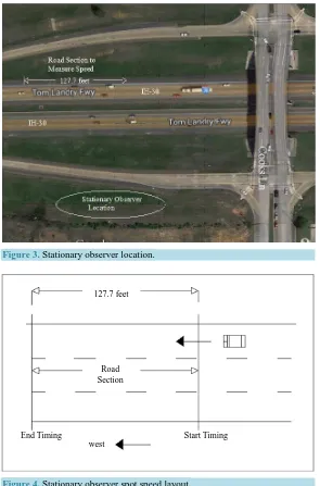
The observer’s location must be higher than the road section to have a dominant view of the roadway as shown inFigure 3. In this case, the observer stood on a hill beside a bridge, looking down on the road segment under study. A reference point was utilized to help in collecting the amount of time it takes a vehicle to travel across the road section by the observer. In this project the reference point to start timing was a vertical stake and the reference point to end timing was a signpost, as shown schematically in Figure 4.

Figure 3. Stationary observer location.

west

Start Timing End Timing

Road Section 127.7 feet

The site used for data collection is the intersection between I-30 and Cooks Ln in the Dallas Fort Worth (DFW) area, Texas. This location is in the middle of the five-mile stretch. Data on the required inputs for esti-mating traffic flow, speed, and density using stationary observer method were collected on the selected location.

Procedure

The stationary method involves the participation of two observers for measuring traffic flow and speed over a selected location. The first observer in the specific location counts the traffic flow. Another observer records the video to measure the speed.

Off-peak periods were used for the data collection on the specific location between 11:45 am and 12:15 pm on Saturday, January 31, 2015. Similarly, all the data were collected during daytime period and good weather conditions (clear and dry 50˚F).

In the chosen location, the observer held a camera recording a video. Real time traffic events over the entire period of the test runs were captured by the video and were stored onto a memory card which used later for processing. The observer played back the recorded traffic events in a computer to extract the required data. During the replay, the observer recorded the total numbers of cars passed during the period for obtaining the flow and measuring the time it requires a vehicle to travel between two points on the road section to estimate the speed. The total numbers of vehicles passed during the half-hour period were found to be 1875, corresponding to an hourly volume of 3750 vph.

A statistical analysis was conducted to verify the adequacy of the sample size used. The equation for deter-mining a minimum sample size was used to achieve a required degree of statistical accuracy according to Equa-tion (5) [3]. Applying Equation (5) for the westbound direction along the road section yields a minimum sample size of 86 observations to achieve a 95% confidence interval. Standard deviation is ±5 mph, and ±1 mph is the permitted error in average speed. These values provide sufficient, reasonable and consistent estimates of speed. Thus, 86 random observations were made for speed measurements.

2 2 2

1.96 N

E σ

= (5)

where,

N = the minimum required number for measuring speeds.

1.96 = the z-value for standard normal curve with 95% confidence interval. σ = estimated sample standard deviation, mph.

E = permitted error in the average speed, mph.

A rolling wheel odometer was used to measure the length of the road section, which was found to be 127.7 feet long. The travel time for each vehicle corresponding to the above segment length was measured. Then the speed was estimated as the ratio of the segment length to the travel time. Table 2presents the speed estimates given by following Equation (6) [3] for each of the 86 vehicles travelled in the study segment of westbound I-30 from: 11:45 am to 12:45 pm on January 31, 2015.

1.47 D V

T

= (6)

where,

V = travel speed, mph.

D = length of the study section, feet. T = elapsed time, seconds.

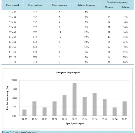
Equation (6) is used to determine the directional spot speed for the westbound segment. Figure 5illustrates the relative frequency percentage for each speed interval, and the speed calculated for each of the 86 vehicles. The space mean speed was found to be 62.1 mph.

4. Statistical Analysis

Table 2.Speed data obtained by stationary observer.

Class interval Class midpoint Class frequency Relative frequency

Cumulative frequency

Number Relative

51 - 52 51.5 3 3%

53 - 54 53.5 7 8% 10 12%

55 - 56 55.5 4 5% 14 16%

57 - 58 57.5 7 8% 21 24%

59 - 60 59.5 10 12% 31 36%

61 - 62 61.5 16 19% 47 55%

63 - 64 63.5 9 10% 56 65%

65 - 66 65.5 11 13% 67 78%

67 - 68 67.5 8 9% 75 87%

69 - 70 69.5 4 5% 79 92%

71 - 72 71.5 7 8% 86 100%

51-52 53-54 55-56 57-58 59-60 61-62 63-64 65-66 67-68 69-70 71-72

Spot Speed (mph) Histogram of spot speed

0.00 5.00 10.00 15.00 20.00

R

el

a

ti

v

e F

req

u

en

cy

(

%

)

Figure 5. Histogram of spot speed.

4.1. Traffic Flow

H0: q (moving observer) = q (stationary observer). HA: q (moving observer) ≠ q (stationary observer).

Then, the test statistic is calculated using the following equation:

statioary

MO calc

q q

t

s n

−

= (7)

(

)

191.3 1

qi q s

n −

= =

−

where;

S = standard deviation. q = arithmetic mean. qi = individual observation. N = total number of observations. Equation (7) yields:

3708 3750 0.54 191.3 6

calc

t = − = −

The degree of freedom is ν= − = − =n 2 6 2 4.

The t-value from the table for ν =4 and at 90% level of confidence is ttable = 2.132. |tcalc| < ttable

We, therefore, fail to reject Ho. This implies that the two means are statistically the same. Additionally the acceptance Region “confidence interval” is:

C.I =

(

)

C.I =

(

)

C.I = (3584 ≤ q ≤ 3916)

We are 90% confident that the mean traffic flow lies between 3584 (vph) and 3916 (vph). Since, using the moving observer method the mean traffic flow is calculated to be 3708 vph, there is no statistical difference be-tween the two means.

4.2. Space Mean Speed

H0: U (moving observer) = U (stationary observer). HA: U (moving observer) ≠ U (stationary observer).

Then, the test statistic is calculated using the following equation:

statioary

MO calc

U U

t

s n

−

= (8)

(

)

1.7 1

Ui U s

n

Σ −

= =

−

63.2 62.1 1.58 1.7 6

calc

t = − =

The degree of freedom is ν= − = − =n 2 6 2 4.

The t-value from the table for ν =4 and at 90% level of confidence is ttable = 2.132.

table

calc t <t

We, therefore, fail to reject Ho. This implies that the two means are statistically the same. Additionally, the acceptance Region “confidence interval” is:

C.I =

(

)

C.I =

(

)

C.I = (61 ≤ U ≤ 63.2)

5. Conclusions

The traffic flow, speed and density are required input variables for the planning, designing, and modelling of the traffic stream for all parts of the road system. In estimating these variables for such applications, it is suggested that the stationary measurements are the most preferred approach for more accurate results. However, the Mov-ing Observer Method yielded reasonably accurate estimates with just two observers and test vehicle.

The main objective of this project has been to compare of the traffic flow and speed using the moving observ-er method to the traffic flow and speed measurements using the stationary obsobserv-ervobserv-er method. The results from the two approaches are statistically compared. Findings from the study revealed that traffic flow values based on the stationary method were found to be (slightly) higher by about 42 vph than those based on the moving observer method. In contrast the speed values based on the moving observer method were found to be slightly lower by about 1.1 mph than those based on the stationary method. These differences were found to not be statistically significant at 90% level of confidence. This confirms the validity of the moving observer method as an effective and accurate method to estimate the traffic flow and speed.

The most attractive feature of using the moving observer method is an inexpensive means to obtain the traffic flow and speed simultaneously. It is therefore an economical method since the total amount of man power and hours needed to attain a high level of accuracy is smaller for the moving observer method compared to the sta-tionary method.

The two methods have been collected on the same day Saturday, January 31, 2015 from (11:00 am-1:00 pm). The weather was clear and dry (50˚F - 60˚F) on the observation day. Therefore, the influence of weather on traf-fic variables was negligible.

Even a higher level of accuracy can be reached by considering the following:

 Enlarging the sample size or increasing the number of runs.

 Segmenting the measurements by the type of vehicle, since traffic flow and speed could have different val-ues for different vehicle types.

 Studying different scenarios with different number of lanes and at different times of day (peak, mid-peak, off-peak).

References

[1] Wardrop, J.G. and Charlesworth, G. (1954) Method of Estimating Speed and Flow of Traffic from a Moving Vehicle.

Proceedings of the Institution of Civil Engineers, 3, 158-169. http://dx.doi.org/10.1680/ipeds.1954.11628

[2] O’Flaherty, C.A. and Simins, F. (1970) An Evaluation of the Moving Observer Method of Measuring Traffic Speeds and Flows. Australian Road Research Board, 40-54.

[3] Robertson, H.D., Hummer, J.E. and Nelson, D.C. (1994) Manual of Transportation Engineering Studies. Institute of Transportation Engineering, Englewood Cliffs.

[4] Mortimer, W. (1957) Moving Vehicle Method of Estimating Traffic Volumes and Speeds. Highway Research Board, 156, 14-26.