A Probabilistic Algorithm for Optimal Control Problem
Akbar Banitalebi
Department of Mathematical Sciences, Faculty of Science, Universiti Teknologi Malaysia,
Johor, Malaysia
Mohd Ismail Abd Aziz
Department of Mathematical Sciences, Faculty of Science, Universiti Teknologi Malaysia,
Johor, Malaysia
Rohanin Ahmad
Department of Mathematical Sciences, Faculty of Science, Universiti Teknologi Malaysia,
Johor, Malaysia
ABSTRACT
In this paper we present a direct method for the numerical solution of the constrained optimal control problem when the gradient information is not available. At this aim, a new control parameterization based on Bernstein basis functions is suggested to convert control problem into nonlinear programing problem (NLP), and then a recently proposed stochastic algorithm called Probabilistic Global Search Johor (PGSJ) is considered for the solution of resultant NLP. The underlining idea of the PGSJ algorithm is to use probability density functions (PDF) to direct the search while no recombination operator is used. This algorithm along with the new Bernstein-based control parameterization (BCP) is compiled into BCP/PGSJ direct method to be applied to approximate the solution of the control problem up to the accuracy required. This method is lastly implemented while simulating some case studies which illustrate the efficiency of the method.
Keywords
Optimal Control Problem, Constraints, Direct Methods, Stochastic Algorithm.
1.
INTRODUCTION
The optimal control problems frequently arise in many areas of science, engineering, management, finance etc. Typical applications often occur when natural or artificial processes are mathematically modeled by system of nonlinear ordinary differential equations involving input and output variables respectively known as control and state variables. In this case, the problem objective is generally to identifying the best control variables to optimize a designed performance index. This paper is aimed at addressing a general class of the aforementioned problems with the objective of approximating the best control function that minimizes a performance index of Mayer type (tf )for any real-valued bounded function while the interaction between control and state variables is governed by
( ) ( ( ), ( ), ), x t f x t u t t
with initial value x t(0)x0,and the constraint of the problem is described by
( ( ), ( ), ) 0 g x t u t t
where x indicates the state function on the time interval
0 f
t t t into the n-dimensional Euclidean space,uis the control curve on the same time interval into a box subset of the form[ , ] [a b1 1a b2, 2] [am,bm]Rm, and lastly
f andg are functions on RnRmR into Rn and
q
R respectively.
The optimization of this problem has become a multidisciplinary research area in virtue of numerous applications in a variety of areas. However, the analytic solution for this problem is only available for few relatively simple cases, and therefore investigation into numerical approaches to approximate an accurate enough solution for arising problems is inevitable. In addition, as no method is without its own disadvantages, the need for more practical methods has not shown any sign of abating.
The existing numerical methods available in the open literature are usually divided into three classes, dynamic programing methods, indirect or variational methods, and direct methods.
The idea of dynamic programing was first introduced in the middle of the last century [1] and later developed into the Bellman principle of optimality [2, 3]. Methods based on this principle however, are often inefficient when problems are of high dimension. The efforts to address this drawback led to the development of iterative dynamic programing (IDP) [4]. Apart from Bellman principle, the Pontryagin minimum principle [5] was also developed almost concurrently, and subsequently many more necessary and sufficient conditions for optimality derived [6, 7]. Algorithms based on these principles usually enforce computing some new variables known as co-states using gradient information, and then these intermediate variables help to obtain the actual ones, hence why these methods called indirect.
Many effective algorithms already exist based on the aforementioned principles however it is sometimes prohibitive to use them efficiently due to complexity of arising problems when problems are singular, nonsmooth, highly nonlinear or multimodal. In these cases, the direct methods seem to be the more practical alternative.
These methods typically use a discretization technique to transfer the control problem to a nonlinear programing problem (NLP), and then a suitable NLP solver is employed to solve the converted problem. The direct methods can also be classed into stochastic and deterministic approaches, depending on the search strategies applied.
search (CRS) [11], Partial Swarm Optimization (PSO) [12, 13], Evolutionary Algorithm (EA) [14], Line-up Competition Algorithm (LCA) [15], and ecologically inspired methods [16] are already applied on optimal control problems. In this study a recently proposed algorithm called Probabilistic Global Search Johor (PGSJ) [17] is considered for the numerical solution of previously mentioned control problem. The next section includes a description of PGSJ. In the third section the Bernstein-based control parameterization (BCP) and its advantages are discussed. Subsequently, the BCP/PGSJ direct method is evaluated while applying on some case studies collected from the literature, and finally conclusion is included in the last section.
2.
PGSJ ALGORITHM
This algorithm has been developed [17] for global optimization problems of the following form,
min ( )f (1)
where f is a real-valued bounded function, andis a box subset[ , ] [a b1 1a b2, 2] [a bn, n]inRn.The main feature
of PGSJ algorithm is to carefully sampling among feasible points in the search space in accordance with some probability density functions (PDFs) which are uniformly initialized. These PDFs are then iteratively biased toward optimal solution, while no recombination operator as it is customary in GA and EA algorithms is employed. The details of the algorithm are subsequently described.
2.1
Algorithm Initializations
[image:2.595.319.535.113.239.2]In order to facilitate starting the algorithm first some input functions and parameters have to be provided which are briefly outlined below and explained in the subsequent subsections. At this aim, the symbols appear in the first column of Table 1 are defined as the corresponding meaning in the next column.
Table 1. The algorithm inputs n Dimension of the problem,
f The Objective function,
D The box [ , ] [a b1 1a b2, 2] [a bn, n],
N The number of partitions on each interval, S The number of samples in each iteration, A The acceptable probability density, b The number of bisecting procedure,
The Scale Factor, I Increment in probability,
The accuracy required,
m Maximum Number of iterations,
P Probability of sampling from complementary search space.
After reading above inputs, each interval [ ,a bi i]is partitioned intoN subintervals, a complementary search space is initialized as an empty set, and then a PDF iof the
following form is initialized uniformly for each intervali.
1
( ) ( )
ij n
i ij I
j
t p t
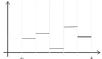
for ai t bi (2)whereIijis the thj subinterval on [ ,a bi i], indicates the characteristic function, and parameterspij first initialized
equally as it is shown in Figure 1.
Fig. 1: The graph of iat initializing point withN 5. The next stage of the algorithm is four nested loops. The innermost loop invokes sampling procedure where new trial solutions are sampled.
2.2
The Sampling Loop
[image:2.595.340.513.424.524.2]This part of algorithm is designed for samplingS new points from the search space according to PDFs. At the first try, sampling is done according to a uniform distribution, and then it just the matter of generating random points uniformly. However, in subsequent iterations as PDFs iteratively are updated, distributions in sampling task are no longer uniform. In addition, some regions of search space are iteratively added to the complementary search space and need to be dealt separately. Therefore, different strategy has to be applied for sampling in accordance with a general PDF as illustrated in Figure 2.
Fig. 2:An illustration of a general PDF of the form (2). In order to sample a general PDF, a common approach is to use the inverse of cumulative density function (CDF) related to the PDF along with a uniform pseudo-random point generator. Therefore to put this idea into practice, namely to generate one point according to the PDF (2), if the complementary search space is not empty, with probability P a point is sampled from this region, otherwise a random number 0 1 is uniformly generated. This number has to be satisfied in one of the following conditions,
1
1
0 n
i i
p p
(3)1
1 1
1 1
j j
i i
i i
n n
i i
i i
p p
p p
[image:2.595.50.286.494.648.2]when condition (3) satisfies, a point uniformly samples from the first subinterval, otherwise if condition (4) for 2 j n satisfies, the thj subinterval uniformly samples. This procedure then helps to sample a point according to PDF (2). AfterSpotential solutions sample, the next loop update the PDFs.
2.3
Probability Updating Loop
The trial solutions sampled in the previous loop are evaluated in this loop, and then the best and the worst trials help to update PDFs. For each intervali,pijin PDF (2) decreases
topijpijI if the worst trial locates in thj subinterval, andpikincreases to pik pijI if the best trial found to be
in the thk subinterval. The same procedure in this loop repeats until the following condition is satisfied,
0 0
,
ij i n j N
min max p A
(5)
and then, the next nested loop is started which is described in the next subsection.
2.4
Partitioning Loop
After a few cycle of probability updating loop, the best subinterval as well as the worst subinterval in each interval can be identified. Each partitioning loop remove the worst subintervals from the search space and adds them to a complimentary search space, and then bisects the best subinterval to retain the number of subintervals while sharing the probability related to both best and worst subintervals between new subintervals equally. Figure 3 illustrates a PDF after one cycle of this partitioning loop. This loop is cycled
[image:3.595.334.520.112.233.2]forbtimes, and hence we arrive at the outermost loop where the algorithm restarts the search to focus search efforts on the most promising region.
Fig. 3:An illustration of a PDF after one cycle of partitioning loop.
2.5
Restarting Loop
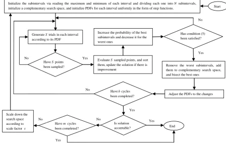
The previous nested loops of the algorithm are designed to avoid getting trap in local solutions while the outermost loop is to speed up the search by scaling down the search space centered at the best solution found so far using the scale factor. Then the removed regions of search space are again added to the complementary search space. The new intervals in the new search space are again partitioned into N subintervals. Simultaneously, all PDFs are adjusted to the change by reinitializing them uniformly on the new intervals. This loop is run until either the best solution arrives at a neighborhood of global solution of radiusor the number of restarting cycles exceedsm. The whole procedure described above, is illustrated in Figure 4, where the algorithm is depicted using a flowchart diagram.
Fig 4: The PGSJ flowchart
Initialize the subintervals via reading the maximum and minimum of each interval and dividing each one intoN subintervals, initialize a complementary search space, and initialize PDFs for each interval uniformly in the form of step functions.
GenerateStrials in each interval according to its PDF
HaveSpoints been sampled?
EvaluateSsampled points, and sort them, update the solution if there is improvement
Increase the probability of the best subintervals and decrease it for the worst ones
Has condition (5) been satisfied?
Remove the worst subintervals, add them to complementary search space, and bisect the best ones
Adjust the PDFs to the changes Havebcycles
been completed?
Is solution
acceptable? End Havemcycles
been completed? Scale down the
search space according to scale factor s
Start
No
Yes
No Yes
Yes
Yes
No No
[image:3.595.57.506.450.744.2]3.
DISCRETIZATION
As with many other NLP solvers, the PGSJ algorithm is only applicable to handle finite dimensional optimization problems. However, the solution of the previously described continuous time control problem actually requires identifying an infinite number of unknowns. Therefore, the original control problem has first to be converted into Problem (2). There are two common frameworks to directly convert a control problem into an NLP problem. They are complete discretization and control parameterization.
In the complete discretization also known as simultaneous approach [18], the whole variables of an optimal control problem discretized reducing the need for online solution of initial value problem; however this converts the original problem into a very large scale NLP problem.
On the other hand, in the control parameterization approach only the control functions are parameterized. The basic idea is to approximate these functions by a liner combination of a basis function with unknown coefficients. The resultant NLP problem of identifying the best values for related coefficients is then usually of relatively smaller scale. In addition, the state functions are not parameterized. Hence, better approximation for these functions.
These advantages help the control parameterization to be a popular framework in the direct solution of practical control problems. A variety of basis functions have been used in this framework, including piecewise constant functions [19, 20], piecewise linear functions [12, 14], Chebyshev polynomials [21], B-splines functions [22], Lagrange polynomials [23], Legendre wavelets [24], and Bézier curves [16].
In this work we introduce a new approach for parameterization of the control function based on Bernstein basis function [25] which suggests a very efficient means of function approximation. The same basis function used in [16] to parameterize control function, however the suggested parameterization has the advantage that time interval does not need to be discretized. The approximated control is shown below, 0 0 0 ! ( ) ( ) ( ) !( )! ( )
n i n i
i
f n i
f
n u
u t t t t t
i n i
t t
(6)wherenis an arbitrarily chosen positive integer. The larger value is chosen forn, the more accurate solution is obtained for controlu. This value actually indicates the number of unknown coefficients ui (fori 1,n) that need to be
identified. This Bernstein-based control parameterization (BCP) is employed in the next section while studying some case studies. After converting control problem into NLP problem, resultant problem is solved using the PGSJ algorithm while the explicit Runge–Kutta method [26] is used to integrate the related initial value problem.
4.
CASE STUDIES
In order to evaluate the efficiency of BCP/PGSJ direct method the PGSJ algorithm [17] along with BCP parameterization technique as well as Runge–Kutta method [26] are coded
using C++/Cli programming language. The new method is then implemented on some typical problems while the control functionuis approximated by polynomial of the form (6) withn5. Additionally, only 40000 function evaluations is allowed while running PGSJ, and the main parameters are set as follow, N 7, S 50, A0.5, b5, and 0.9.
4.1
A Biological Case
The first problem is of the linear quadratic form. It is based on a biological model and selected from [16, 27].
2 1 1 2 2 2 1 (1) ( ) ( ) ( ) ( ) 3 ( ) ( )
min J = x
x t x t u t
x t x t u t
The exact analytic solution for this problem is available through applying Pontryagin's minimum principle [5]. This problem is solved using BCP/PGSJ to assess the performance of this method against this exact analytical solution.
4
2 2
4 4
4
* 2 2
1 4 4
8 8
* 4 4
2 4 2 4 2 4 2
3 3
( )
3 1 3 1
3 3
( )
3 1 3 1
9 3 3(1 3 )
( )
(3 1) (3 1) (3 1)
t t
t t
t t
e
u t e e
e e
e
x t e e
e e
e e
x t e e
e e e
In this circumstance, the method obtains a solution of 2.791 for this problem. The results of the computations are compared and depicted in Figure 5 and Figure 6.
Fig. 5: Control functions related to the case study 4.1.
4.2
Continuous Stirred Tank Reactor
Problem
The second case study is a chemical process which has been modeled [28] by the following nonlinear differential equations.
1
1 1 2 1
1
1
2 2 2
1
2 2 2
3 1 2
25
( 0.25) ( 0.5) exp( ) (1 )( 0.25) 2
25
0.5 ( 0.5) exp( )
2 0.1
x
x x x u x
x x
x x x
x
x x x u
The objective of this problem is to minimize the value of 3(f )
Jx t whiletf 0.78, the initial value assumed to be (0) [0.09,0.09,0.0]T
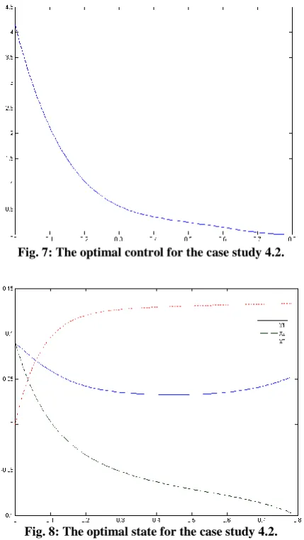
[image:5.595.310.535.144.251.2]x and 0u t( )5for 0 t 0.78. This problem appears in the list of benchmark problems collected in the hand book of test problems [29]. It is a multimodal problem having a local solution of J 0.2442and a global one J0.1330 [13, 28].
Fig. 7: The optimal control for the case study 4.2.
Fig. 8: The optimal state for the case study 4.2.
According to a comparative study [14], some EA methods may acquire the solution of 0.1355 at reasonable computational efforts while using IDP, it is still likely to trap into the local solution. Sun et.al, [15] also solved this problem where the best solution obtained is 0.1332 at approximately 40000 function evaluations. With the same parameter setting
as in 4.1 the BCP/PGSJ algorithm obtains the average solution of 0.1334, and the best solution of 0.1332. Table 2 shows the number of function evaluations while this problem is being solved, and the graphs of optimal control and states related to this solution are as in Figure 7 and 8.
Table 2. Solution of the case study 4.2 using BCP/PGSJ Iteration Function evaluation Value of J
5 2665 0.2282
15 7982 0.1748
25 13223 0.1657
35 18671 0.1541
45 23987 0.1463
55 29312 0.1403
65 34645 0.1373
75 39971 0.1332
4.3
State Constrained Control Problem
The next problem is modeled by the following differential equations,1 2
2 2
2 2 2
3 1 2
4
0.005 1
x x
x x u
x x x u
x
The initial value for this problem is (0)x [0, 1,0,0] T , while the constraint is determined by,
2 1( ) 8( 4( ) 0.5) 0.5 0
x t x t for 0 t 1. The objective of this problem is to minimize the value of
3(f )
x t whiletf 1, and the control function is bounded by 5 u t( ) 15 . In order to handle this constraint a new state variable is introduced to the above system of differential equations.
2 5 max(0, 1 8( 4 0.5) 0.5)
x x x
with the initial value at x5(0)0. In addition, the performance index is also augmented with a penalty factorx t5(f )where the penalty parameteris any large
enough number. The objective of the problem is then equal to minimizing
3(f ) 5(f )
x t x t .
This problem has been solved by Neuman and Sen [30] using cubic splines.
Vlassenbroeck
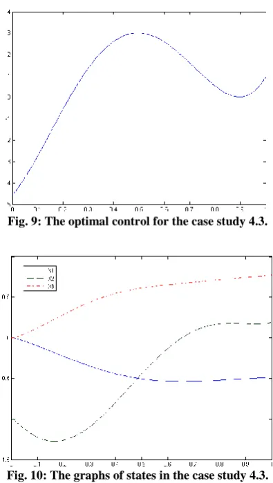
[21] has also applied a Chebyshev polynomial method where the best solution is 0.74096 . [image:5.595.60.275.302.684.2]function evaluations which results in the solution of 0.7539. In the second attempt we used up to 80000 function evaluations, andn6to attain the solution of 0.7409
[image:6.595.67.265.116.466.2]Fig. 9: The optimal control for the case study 4.3.
Fig. 10: The graphs of states in the case study 4.3.
4.4
Rayleigh's problem
The forth problem is also a continuous inequality constraint control problem collected from [19] which is described by the following system of differential equations
1 2
2
2 1 2 2
2 3 2 1
(1.4 0.14 ) 4
x x
x x x x u
x u x
while the inequality constraint being
1 1
( ) ( ) 0
6
u t x t for 0 t 4.5
the initial value at x(0) [ 5, 5,0]T and the objective is to minimize the value ofx t3(f )whiletf 4.5.
Using the same constraint handling technique as in previous problem we first define the following differential equation,
4 1 1
1
1 1
( ) ( ) 0
6 6
1
0 ( ) ( ) 0
6
u x u t x t
x
u t x t
with initial value at x4(0)0, and therefore the new augmented performance index is
3(f ) 4(f )
x t x t
where is a penalty parameter.
We use the aforementioned parameter setting for PGSJ algorithm as in first problem and polynomial of degree 5 in BCP parameterization where the best value of 47.6947 is obtained for the performance index. Figure 16 shows that the graph of the constraint never exceeds the vertical axe. Additionally, Figures 12 to 15 illustrate the optimal control, and states which are agree with those results obtained in [19].
[image:6.595.319.536.249.622.2]Fig. 11: The graph of the constraint in the case study 4.3.
Fig. 12: The optimal control for the case study 4.4.
5.
CONCLUSION
method was implemented using C++/Cli programming language which facilitates evaluating this method while some case studies simulated. The results of simulations show the efficiency of the proposed method.
[image:7.595.70.266.135.690.2]Fig. 13: The graph ofx in the case study 4.4.1
Fig. 14: The graph ofx for the case study 4.4. 2
Fig. 15: The graph ofx in the case study 4.4. 3
6.
ACKNOWLEDGMENTS
The authors would like to thank the Malaysian Ministry of Higher Education and Research Management Centre of Universiti Teknologi Malaysia for their support and financial funding through research grant Vot. No. 4B045.
Fig. 16: The graph of the constraint of the case study 4.4.
7.
REFERENCES
[1] Bellman, R.E. 1957. Dynamic Programming. Princeton University Press, New Jersey.
[2] Howard, R.A. 1960. Dynamic programming and Markova processes. The MIT Press, Massachusetts. [3] Bellman, R. 1971. Introduction to mathematical theory
of control processes. vol. 2. Academic Press, New York. [4] Luus, R. 2000. Iterative Dynamic Programming.
Chapman and Hall CRC Press, Florida.
[5] Pontryagin, L.S., Boltyanskii, V.G., Gamkrelidze, R.V., and Mischenko, E.F. 1962. The mathematical theory of optimal processes (Translation by Neustadt L.W.). Macmillan, New York.
[6] Hartl, R.F. 1984. A survey of the optimality conditions for optimal control problems with state variable inequality constraints. In Brans, J.P. (Ed.) Operational research '84. (pp. 423-433). North-Holland, Amsterdam. [7] Hartl, R.F., Sethi, S.P., and Vickson, R.G. 1995. A
Survey of the Maximum Principles for Optimal Control Problems with State Constraints. SIAM Review, 37(2), 181-218.
[8] Carrillo-Ureta, G.E., Roberts, P.D., and Becema, V.M. 2001. Genetic algorithms for optimal control of beer fermentation. Proceedings of the 2001 IEEE, International Symposium on Intelligent Control September 5-7, 2001 Mexico City, Mexico.
[9] GirirajKumar, S.M., Rakesh, B., Anantharaman, N. 2010. Design of controller using simulated annealing for a real time process. International Journal of Computer Applications, 6(2), 20–25.
[10]Babaeizadeh, S., Banitalebi, A., Rohanin, A., and Mohd-Ismail B.A.A. 2011. An ant colony approach to optimal control problem. International Seminar on the Application of Science & Mathematics 2011. PWTC, Kuala Lumpur, Malaysia.
[11]Ali, M.M., Khompatraporn, C., and Zabinsky, Z.B. 2005. A Numerical Evaluation of Several Stochastic Algorithms on Selected Continuous Global Optimization Test Problems. Journal of Global Optimization, 31, 635– 672.
[13]Kumar, R.K., Anand, S. and Sydulu, M. 2012. A Novel Multi agent based PSO approaches for security Constrained Optimal Power Flows using smooth and non-smooth cost functions. International Journal of Computer Applications, 41(3), 14-21.
[14]Cruz, I.L.L., Willigenburg, L.G.V., and Straten, G.V. 2003. Efficient Differential Evolution algorithms for multimodal optimal control problems. Applied Soft Computing, 3, 97–122.
[15]Sun, D.Y., Lin, P.M., Lin, S.P. 2008. Integrating controlled random search into the line-up competition algorithm to solve unsteady operation problems. Industrial & Engineering Chemistry Research, 47, 8869– 8887.
[16]Ghosh, A., Das, S., Chowdhury, A., Giri, R. 2011. An ecologically inspired direct search method for solving optimal control problems with Bezier parameterization. Engineering Applications of Artificial Intelligence, 24, 1195–1203.
[17]Banitalebi, A., Mohd-Ismail B.A.A., and Rohanin, A. 2011. A new probabilistic global search algorithm. Regional Annual Fundamental Science Symposium 2011, Thistle Hotel, Johor, Malaysia.
[18]Biegler, L.T. 2007. An overview of simultaneous strategies for dynamic optimization. Chemical Engineering and Processing, 46, 1043–1053.
[19]Loxton. R.C., Teo, K.L. Rehbock, V., and Yiu, K.F.C., 2009. Optimal control problems with a continuous inequality constraint on the state and the control. Automatica, 45, 2250-2257.
[20]Goh. J., Teo, K.L., 1988. Control parameterization: a unified approach to optimal control problems with general constraints. Automatica, 24(1), 3–18.
[21]Vlassenbroeck, J. 1988. A Chebyshev Polynomial Method for Optimal Control with State Constraints. Automatica, ( 24) 4, 499-506.
[22]Schlegel, M., Stockmann, K., Binder, T., Marquardt, W. 2005. Dynamic optimization using adaptive control vector parameterization. Computers and Chemical Engineering (29) 1731–1751.
[23]Biegler, L., 1984. Solution of dynamic optimization problems by successive quadratic programming and orthogonal collocation. Computers and Chemical Engineering. 8 (3–4), 243–248.
[24]Sadek, I., Abualrub, T., Abukhaled, M. 2007. A computational method for solving optimal control of a system of parallel beams using Legendre wavelets. Mathematical and Computer Modeling, 45, 1253–1264. [25]Farouki, R.T., and Rajan, V.T. l988. Algorithms for
polynomials in Bernstein form. Computer Aided Geometric Design, 5, l-26.
[26]Tsitouras, Ch. 2011. Runge–Kutta pairs of order 5(4) satisfying only the first column simplifying assumption. Computers and Mathematics with Applications. 62, 770-775.
[27]Lenhart, S. and Workman, J.T. 2007. Optimal control applied to biological models. Mathematical and Computational Biology Series. Chapman and Hall, CRC Press, Boca Raton.
[28]Kirk, D.E. 1970. Optimal Control Theory: An Introduction. Prentice Hall Inc. New Jersey.
[29]Floudas, Christodoulos A. 1999. Handbook of test problems in local and global optimization. Kluwer Academic Publishers. Dordrecht.