A Time-minimization Dynamic Job
Grouping-based Scheduling in Grid Computing
Manoj Kumar Mishra
School of Comp. Engg. KIIT UNIVERSITY, Bhubaneswar, Odisha, India
Prithviraj Mohanty
School of Comp. Engg. KIIT UNIVERSITY, Bhubaneswar, Odisha, India
G. B. Mund
School of Comp. Engg KIIT UNIVERSITY, Bhubaneswar, Odisha, India
ABSTRACT
Grid computing is the novel framework that offers a flexible, secure and high performance computing, on demand for solving high compute-intensive applications with large number of independent jobs. However, user jobs developed for grid might be small and of varying lengths according to their computational needs and other requirements. Certainly, it is a real challenge to design an efficient scheduling strategy to achieve high performance in grid computing. But there exists some grouping based job scheduling strategy that intends to minimize total processing time by reducing overhead time and computation time, and on the other hand maximizing resource utilization than without grouping based scheduling. The purpose of the study is to analyze and achieve better performance by extending the concept of grouping based job scheduling. Therefore, this paper proposes “A Time-Minimization Dynamic Grouping-Based Job Scheduling in Grid Computing” with the objective of minimizing overhead time and computation time, thus reducing overall processing time of jobs. The work is verified through various observations made in different simulated grid environments. The results obtained shows that the proposed grouping-based scheduling algorithm is on average, comparable to, or even better than, other grouping based scheduling algorithms.
Keywords—
Grid computing; Job grouping; Job scheduling
1.
INTRODUCTION
The idea of Grid Computing was first envisioned by Leonard Kleinrock in 1969, when described: “like electric and telephone utilities, spread of computer utilities will service individual homes and offices across the country” [1, 2]. The term “Grid” was used during mid-90’s to symbolize a proposed distributed computing infrastructure for advanced science and engineering projects [3]. The word “Grid” refers to systems and applications that integrate resources and services distributed across multiple control domains. Computational grids provide large-scale resource sharing, such as personal computers, clusters, MPPs, Data Base, and online instructions, which may be cross-domain, dynamic and heterogeneous [4]. If one considers the internet as a network of communication, grid computing can be considered a network of computation [5]. Grid offers a next generation high performance computing platform analogous to a power Grid that supplies consistent, pervasive, dependable, transparent access to electricity irrespective of where it is generated [6]. And its development involves sharing, exchange, discovery, aggregation, selection and efficient management of resources distributed across multiple administrative domains, organizations and enterprises. This enables the users to compute large scale applications in science, engineering and business, by utilizing the increased
access to geographically spread and dynamically available processing powers, storage devices, data, computational services, scientific instruments, and other computational resources. This paper defines “Grid Computing” as an abstraction that provides a high performance computing environment by offering transparent, scalable, economical and authorized resources to the registered users on demand, hiding most of its underlying details and complexities from the outside world.
capabilities of the available resources, and proceed with the job scheduling and deployment activities [9]. This grouping based job scheduling strategy reduces communication time resulting increase in computation-communication ratio (CCR), which encourages distributing grouped jobs for processing on remote resources [10]. But it is yet to be tested where jobs may be fine-grained but their length differs considerably from one another. And scheduling can be done when one resource or more than one resource is available at the time of scheduling. Hence, scheduling should be addressed by developing a grouping strategy suitable to both type of grid environment. The motivation of this paper is to develop an enhanced grouping based job scheduler and grid resource allocation algorithm that must be efficient and effective in reducing the total processing time of jobs. The rest of this paper is organized as follows. Section 2 analyzes related works in the field of parallel and distributed memory system and grid computing systems. Section 3 describes the grid system and scheduling components (broker). Section 4 presents proposed dynamic grouping-based job scheduling model. Section 5 analyses simulation results made through various observations and section 6 gives conclusion and future work and lastly, the references.
2.
RELATED WORK
In this section, some of the representative research works on job scheduling in parallel and distributed computing systems and Grid computing environment have been reviewed to explore the relevance of these works.
Sarkar’s algorithm (1989), addresses the scheduling problem of a given directed acyclic weighted graphs (DAG’s) on unbounded number of completely connected processors. Sarkar proposed a two-step method for scheduling with communication. (1) Perform clustering i.e. mapping of the tasks of a DAG onto clusters, with the constraint that all tasks in a cluster must execute in the same processor. (2) Merge and schedule the clusters when the number of processors is smaller than the number of clusters. Sarkar’s primary goal is the minimization of the parallel time cost function on an unbounded number of processors[11]. Likewise, in scheduling Directed Acyclic Graph (DAG) on multiprocessors, as reported in Gerasoulis and Yang (1992), tasks are grouped into clusters to reduce communication and dependencies among them. The intention of this clustering is to reduce the inter-task communication and as a result, time for parallel execution is minimized [12]. The paper by Yang and Gerasoulis (1994) has addressed the scheduling problem of a given directed acyclic weighted graphs (DAG’s) on unbounded number of completely connected processors. The parallel time in executing a clustered DAG is determined by the critical path of the scheduled DAG, called dominant
sequence (DS), which is different from the critical path of the
clustered DAG. The main idea behind the DSC algorithm is to perform a sequence of edge zeroing steps with the goal of reducing the length of a DS at each step. The objective of this scheduling is to allocate tasks onto the processors and then order their execution so that task dependence is satisfied and parallel time is minimized. GLB by Radulescu, A. and van Gemund, A. (1998) describes a new approach for cluster mapping step, called Guided Load Balancing scheduling algorithm for distributed-memory systems and is intended as a second step in the multi-step class of scheduling algorithms. In such a method, three steps can be defined: (1) clustering, (2) cluster mapping and (3) task ordering. ). GLB is a compile time scheduling algorithm for distributed-memory systems [13]. In distributed memory systems, tasks are also grouped together to reduce communication and processing time as
presented in James, Hawick and Coddington (1999) [14]. In grid computing, there are some works on grouping based job scheduling as discussed below. The work in Buyya, Date, et. al. (2004), attempted to reduce overhead time while scheduling large number of fine-grained jobs onto remote resources for analyzing massive data generated in medical science to study human brain activity. In order to eliminate the overhead associated with fine-grained tasks, coarse-grained jobs or meta-jobs are created by gathering a suitable number of jobs at the user-level, and submitting these gathered jobs to the scheduler for deployment [15]. The scheduling strategy in [15] creates significant programming burden on the application developer. The shortcoming of the approach in [15] encourages the authors N. Muthuvelu, Junyan Liu et. al. (2005) to suggest of creating course grained jobs at the scheduling level rather than at programming level. The approach is to group the jobs at the scheduling level according to the processing capabilities of the available resources reducing the transmission overhead and maximizing the resource utilization [16]. The paper by Ng Wai Keat, Ang Tan Fong, (2006) investigates the use of bandwidth-awareness and job grouping concept in a scheduling framework to improve the performance of job scheduling. The Bandwidth-aware scheduling schedules the jobs by considering both computational capabilities and the communication capabilities of the resources. It uses network bottleneck bandwidth of resources to determine the priority of each resource. The scheduler selects the first resource according to its priority and groups independent fine-grained jobs together based on chosen resources processing capability. These job groups are formed to maximize the resource utilization and to reduce network latency [17]. In Quan Liu, Yeqing (2009) Liao, the fine-grained jobs are grouped into forming coarse-grained jobs and allocated to the available resources according to their processing capabilities in MIPS and bandwidth in Mb/s. The grouping algorithm integrates Greedy algorithm and FCFS algorithm to improve the processing of Fine-grained jobs. Algorithm maximizes the resource utilization and reduces the total processing time [18]. The work by M.K.Mishra, R. Sharma, et. al. (2010) mainly focuses on grouping based job scheduling taking into account memory constraint, expected execution and transfer time at the job level rather than at group level in grid system. It supports dynamic grid environment and reduces processing and communication time. It is low cost algorithm and complexity is bounded by О(nlogn) [19].
This study focuses and evaluates an extension to dynamic job grouping based scheduling, which aims to reduce overall processing time of applications by minimizing the job allocation overhead and computation time.
3.
THE GRID SYSTEM: A GENERIC
VIEW
3.1
Grid-Model
A generic grid computing system infrastructure G in this work is assumed to be the collection of R heterogeneous resources and participation of set of U users connected over high-speed interconnection networks. More formally, the collection of resources is represented as {R1, R2…, Rr}. Each resource Ri
owns a set of computing nodes, represented as R= {C1, C2…,
Cc} and belongs to a local domain, i.e. a LAN (Local Area Network). Each computing node Cj is composed of a number
of processors Pk and represented as C= {P1, P2…, Pp}.Where
computers. Multiprocessor systems are defined as computer systems that have several processors sharing a single set of peripherals including the memory. These processors are not autonomous. Distributed Computing Systems, consist of several autonomous processors having their own operating system, with their own local policies. A single processor system or SMP type grid resource provides time-shared environment and the distributed memory multiprocessor systems such as clusters provides a space-shared environment. A cluster/multiprocessor system consists of P processors and let the computation speed of processor j is equal to mj units. A
common unit for measuring capacity can be specified in terms of the rating of standard benchmarks such as million of instruction per second (MIPS) and SPEC. The total capacity
of a computing node is defined as Ci in
p
1
k
P
k
M IPS
and that of Grid resource is defined as Ri in
c
1
j
j
C
M IPS
The Grid Scheduler: The main objective of a scheduler in
most systems often is to design a scheduling policy for mapping of submitted jobs to the resources with the goal of maximizing throughput, efficiency, resource utilization, minimizing job completion times, communication overhead and cost or both time-cost etc. In order to achieve the above mentioned objective in high performance computing environment like Grid should provide a comprehensive and versatile environment and a well defined set of steps to tackle the process of scheduling [20], which is described in the following steps:
Resource discovery: One of the most and first important
goals of the scheduler is to identify a list of authorized resources that can be made available to the registered users.
Grid Information Service: Most Scheduling algorithms
interact with grid information service (GIS) to obtain the initial list of authorized resources, called resource pool. Some of these resources might be meeting the certain minimum requirements of the application such as hardware platform, operating system, RAM or secondary storage space, etc.
Resource selection: Once the information regarding the
available resources in the resource pool is obtained, the next task of the scheduler is to select those resources that are expected to meet time, cost or both time-cost and any other additional constraints enforced by the user. To facilitate user’s requirements the scheduler has to gather dynamic information about resource accessibility, system workload, network performance, and price of the resources etc. Economic environment, like GRACE (Grid Architecture for Computational Economy) [21] offers a set of trading protocols, which enables users and resource owners to negotiate the cost according to the expected starting time, the usage period, the amount of memory or storage requirement etc.
Job scheduling: The job scheduling problem is defined as the
process of making decision for scheduling set of independent jobs onto best possible matching dynamic resources and services that satisfies requirements of jobs and the constraints imposed by users. In grid computing environment, this is the stage where jobs of applications are allocated to selected physical resources based on user’s requirement, resource availability and grid facilities. The scheduling in grid environment has to satisfy a number of constraints on different problems. So,optimal scheduling is a NP-complete problem [7] and different heuristics may be used to reach an
Fig 1: Resources connected across network
[image:3.595.314.544.69.219.2](R denotes combined resources in MIPS available in a cluster)
Fig 2: The Grid Model
optimal or near-optimal solution [22]. In user’s point of view, the objective of the scheduling can be classified into three different categories as minimizing processing time or minimizing cost or both and similarly in resource’s point of view, goal of resource allocation is to optimize the use of resources, maximize the revenue or both. For example, the Nimrod/G broker [23] permits the users to specify a budget constraint, a deadline constraint, or both, and also it incorporates three adaptive scheduling algorithms for cost
- - -
R R
R R
The Internet
SMP
(Cluster)
Cluster
(SMP)
One processor system
INTERNET
GRID BROKER
Rr R1
R
1
RESOURCE LAN
C1 Cc
P1 Pp P1 Pp
optimization, time optimization, or conservative time optimization, within given time and budget constraints.
Monitoring and reliability: Geographically diverse and
dynamic nature of grid makes it difficult to reach the objectives where environmental conditions are subject to unpredictable changes such as system or network failures, system performance degradation, addition or deletion of machines, variations in the cost and computing capability of resources, etc. That is why, it is most important to monitor the tasks running on the nodes of the grid over time and to check reliability factors.
Designing of the Scheduler: Grid scheduling problem can
formally be represented by a set of the given jobs, user and resources. Designing of the scheduler involves matching of application needs of the users with availability of the suitable resources and addressing the concern of the quality of the match. The scheduler design should be meet some predefined and desired objectives, ensuring the quality of service.
Problem Formulation: Applications submitted to the grid
within a time period T consists of several jobs with different characteristics denoted as J = {J1, J2 ,..., Jj}, which do not
require communication with each other and, that belong to a user U = {U1,U2 ,...,Uu},where j≥1and u≥1 . Each job can
necessarily be partitioned into smaller tasks which can run independently in parallel to other tasks and denoted by Tlq, that is, Jl = {Tl1, Tl2, Tl3, .. ., Tlt}. Where l specifies the job-id and is greater than 1, and t ≥1. Applications developed for grid environment can be described by a set of Jl independent jobs with associated workloads, expressed in millions of instructions (MI) and a set of R resources with associated speed, expressed in million instructions per second. In this case, the jobs are grouped according the ability of the remote resources. Also, matching job groups are to be dispatched onto the suitable resources, with the objective of minimizing overhead, processing time of the jobs and maximizing resource utilization. The localized communication cost among the tasks at the resource is assumed to be insignificant in comparison to grid. Thus an instance of the problem consists of a registered user, number of jobs, resources, MI of the jobs and MIPS of the resources.
4.
DYNAMIC GROUPING- BASED
JOBSCHEDULER
The job scheduler is a service that resides in a user machine as depicted in figure 2 and figure 3. Therefore, entire grouping– based scheduling activity can be summarized in the following steps.
Step-1: When the user creates a list of Gridlets or jobs in the user machine, these jobs are sent to the job scheduler for scheduling activity.
Step-2: The job scheduler obtains information about the available registered resources from the Grid Information Service (GIS).
Step-3, 4: Based on this information, the scheduler opts for the resources in line with resource selection strategy. Step-4, 5: The job scheduler prepares job-groups according to the characteristics of selected resources based on the job grouping strategy. The size of a grouped job depends on the processing requirement of individual jobs in the group expressed in Million Instructions. The scheduling process is performed iteratively until jobs and resources are available. Step 6: The grouped jobs are sent to the dispatcher as soon as the jobs are put into various groups based on the schedule made during the matching of jobs with resources.
[image:4.595.313.560.73.487.2]Step 7: The dispatcher then forwards the job-groups to their respective resources for computation. The dispatcher also
Fig 3: Grouping-based job scheduling model
collects the results of the processed jobs from the resources through input ports.
The resource selection along with job-grouping by the scheduler is based on some efficient and low cost strategy agreed upon by both the users and resource providers as described in the following section. The grid structure is illustrated in figure 2 and figure 3 depicts the design of the job scheduler and its interactions with other entities.
4.1 Job Grouping and Resource Selection
Strategy
Grouping of jobs in this paper is based on a resource selection and job grouping strategy. Jobs are grouped according to the ability of the selected resource. Therefore, during job grouping the following conditions must be satisfied:
1
Chunksize
*
IPS
Resource_M
_MI
Groupedjob
2
1
k
where
,
k
1
i
JOB
i
_MI
Groupedjob
Where, MI (Million Instruction) is job’s required computational power, MIPS (Million Instruction per Second) is processing capability of the resources and Chunk_Size is user defined time, used to measure total amount of accumulated MI of jobs that can be completed within a
1 2
222
Gridlet
Scheduler
3
4
4
5
6
7
7
Grid Information Service
User input
Resource Information Table
Gridlets
Grouping strategy
Resources in descending order
Grid resource 1
Gridlet group 1
Grid resource 2
Gridlet group 2
Grid resource r
Gridlet group r Gridlets in descending
order
Gridlet MI Resource MIPS Chunk size
Resource MI Grid Information Collector
Dispatcher Total no of jobs
Average MI rate of job
MI deviation Percentage/without any
particular Deviation Overhead Time
Grid resource 1 Chunk size 1
Grid resource 2 Chunk size 2
specific time window are put together into a group, much like granularity size defined in [9].
To evaluate the total processing time of an application, an analytical performance model is defined in terms of overhead time and computation time of the grouped jobs. Let TCTG, be
the computation time, and TOHT be the overhead time of a
Groupedjob. Therefore,
k
1
i
3
i
t
T
CTGmwhere ti denotes the computation time of jobj of m th
job group, k is the number jobs in the group and executing at resource Rr
satisfying equation 1. The overhead time TOHT of a job group
is the summation of communication time and startup time. Communication time TCOMM is equal to time taken to submit a
group job to resources plus time taken to receive processed Gridlet(s). Likewise, startup time Ts is the sum of time taken
by the scheduler for Gridlet Grouping and the time that elapses between the arrival of the grouped job at the resource and execution start time of the grouped job i.e. local scheduling. The overhead time TOHT is incurred only once at
the group level rather than job level, i.e. in contrast to non grouping based job scheduler.
Hence, overhead time TOHT for mth job group is
4
T
T
T
OHTm
COMMm
sm and processing time of mth grouped job is,
5
T
T
T
PTGm
CTGm
OHTmwhere m≥1. Thus, total processing time of all grouped job is,
6
n
1
m
T
T
TOTAL
PTG
mWhere n is the number of job groups
and
T
CTGm/
T
OHTm1
7
Eq. (7) specifies that overhead time of the grouped jobs should not exceed computation time of the grouped jobs. These are the main parameters to be evaluated to analyze the performance a job scheduler.4.2 The Grouping Strategy
The resources and jobs are sorted out in descending order of their processing power and job length respectively. The resources are taken one after another in FCFS order from the reverse sorted resource list. Once a resource is selected in this manner, jobs are added into job group according to the processing capability of this resource by alternatively taking jobs from front end i.e. job with higher length and then rear end of the job list i.e. job with smaller length. It should be noted that the front end and rear end pointers are updated to point to the next job in the list. While grouping the jobs taken in order of the grouping strategy from the job list, the above strategy falls into one of the two cases given below.
Case1. At some stage in grouping, if given condition in eq. 1 fails, while adding a job into the group from front end of the job list, then it is removed from the group and if possible jobs are taken from the rear end of the list till it satisfies the eq. 1. Case2. If condition in eq. 1 fails while adding a job from rear end of the job list during the grouping operation, then it stops grouping for that resource removing the last job that was added and sends the job group to the dispatcher. Then, it takes next highest resource to perform another job grouping. The above job grouping process is repeated for each resource taken in given order as long as either resources or jobs exist. Fig 4 presents a grouping example.
The purpose of this grouping strategy is as follows. 1) To reduce the overhead time.
2) To maximize number of jobs into the group by taking highest computational resource.
3) To start the grouping process with the addition of a job that involves bigger computational need.
4) To ensure a well combination of bigger and smaller jobs added into the group.
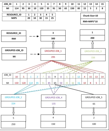
Example:
The proposed job grouping and scheduling algorithm presented next is illustrated through an example. Figure 4 demonstrates an example of job grouping and scheduling scenario where the jobs and resources are created randomly to imitate grid environment. Each job is represented with its JOB_ID and corresponding MI. Similarly each of 5 resources taken is associated with its RESOURCE_ID and corresponding MIPS. These jobs and the resources are sorted out in descending order of their MI and MIPS respectively. In this example 15 user jobs with varying processing requirements (MI) are grouped into five job groups according to the processing capabilities (MIPS) of the available resources and the Chunk_size. Resource MI is calculated as: RMI=MIPS*Chunk_Size and the Chunk_Size is taken as 10. So, the first job-group, i.e. GROUPED_JOB1 is created for the resource with highest MIPS i.e. RESOURCE_ID 3 and MIPS of 30, which is equivalent to MI of 300 taken in FCFS order from the sorted resource list. Before grouping, the job group is initialized to zero. The jobs are added into according to the grouping strategy as mentioned and (the first job is always taken from the front end of the reverse sorted job list i.e. with job-ID 10 and MI 150 is added into the group and total MI of the job group becomes 150, which is less than resource MI of 300. The next is taken from the rear end of the job list i.e. with job-ID 14 and MI of 2 and after adding it to the job list, the total MI becomes 150+2=152, which is still less than 300. Next the third job i.e. the front job with job-ID 5 and MI of 120 is added making the job group 150+2+120=272, which is also less than 300. Then, the next job is added from the rear end of the list i.e. job-ID 13 and job MI of 5, which makes the job group 150+2+120+5=277, it is also less than 300. Then, the fifth job with job-ID 1 and MI of 114 is taken for addition but it becomes greater than 300, so the job is removed from the job group. If possible, the remaining gap between the selected resource and the job group is taken from the rear end only, till it satisfies the equation 1 as mentioned in analytical modeling (the grouping strategy). Therefore, the sequence of jobs with their ID and MI added to job group-1 are <10,150>, <14, 2>, <5,120>, <13, 5>, <15, 8> and <4, 10>. Similarly other job groups i.e. group 2, 3, 4 and 5 are formed according to resources i.e. with resource ID 5, 1, 4, and 2 taken in FCFS order from the reverse sorted list and submitted to the respective resources for computation.
Algorithm:
1. The scheduler receives the Gridlet_List, J [ ] created by the user.
2. Sort the Gridlets according to their Gridlet_Length in decreasing order.
3. The scheduler receives the Resource_List, R [ ]. 4. Sort the Resources in decreasing order according to their
MIPS.
[image:6.595.125.475.83.506.2]
Fig.4 Grouping Strategy: Example
9. //head and tail pointer pointing to the first and last Gridlets in the Gridlet_List respectively.
10. While (Grouped_Gridlet_Length is less than or equal to Resource_MI, R[i] and there are ungrouped Gridlets in the Gridlet_List and unused Resources in Resource_List R[ ] )
BEGIN
10.1– Set Grouped_Gridlet_Length to the summation of previous Grouped_Gridlet_Length and current Gridlet_Length pointed by the head pointer.
- If Grouped_Gridlet_Length is less than or equals to Resource_MI
- update the head pointer. else
-Deduct the last Gridlet added to the Grouped_Gridlet_Length.
- Set Grouped_Gridlet_Length to the summation of previous
Grouped_Gridlet_Length and current Gridlet_Length pointed by the tail pointer.
- If Grouped_Gridlet_Length is less than Resource_MI
- update tail pointer. - Go to step 10.1 else
-Deduct the last Gridlet added to Grouped_Gridlet_Length. -Stop grouping.
END
11. Set a new ID for the Grouped_ Gridlet. 12. Submit the Grouped_Gridlet to Resource, R[i].
13 Increment i (for next resource in Resource-List) and goto step 6.
14 Get the processing time and total Communication Time. Display the details of the processed Grouped_Gridlet to the user through GUI
Explanation:- After receiving the Gridlet list and resource
list, the Gridlets and resources are sorted according to the decreasing order of their MI and MIPS respectively by the
JOB_ID 1 2 3 4 5 6 7 8 9 10 11 12 13 14 15 MI 114 95 30 10 120 35 91 50 65 150 85 15 5 2 8
RESOURCE_ID 1 2 3 4 5 MIPS 20 10 30 15 25
JOB_ID
10 5 1 2 7 11 9 8 6 3 12 4 15 13 14
MI 150 120 114 95 91 85 65 50 35 30 15 10 8 5 2
Chunk Size=10
RMI=MIPS*10
RESOURCE_ID
RMI 200
1
300 3
GROUPED JOB_ID
MI 295 156
GROUPED JOB_1 GROUPED JOB_3
GROUPED JOB_4
224 65
GROUPED JOB_5
135
4
150 5
250
2
100
scheduler (in step-1 to 4). Then, the resources are selected one by one in FCFS order from the reverse sorted resource list and their equivalent MIs are obtained by multiplying with the given Chunk_Size (step-5 to 7). In step-8, and 9, the grouped job MI is initialized to zero and the two pointers head and tail are initialized to point to the first job and last job of the Gridlet list respectively. The grouping strategy is implemented in step 10 and 10.1. While adding and extracting the jobs to and from the group, the head and tail pointers are updated accordingly. In steps 11 and 12, the resource ID will be set for the grouped Job and is sent to the corresponding resource for computation. In step-13, next resource is selected for another grouped job. The above grouping-based scheduling of jobs continues till jobs and resources are available. Steps 14 and 15 generate the report of processing time and communication time after successful execution of the grouped jobs.
5.
SIMULATION ENVIRONMENTS
AND THE RESULTS
GridSim [24] has been used to create the simulation of grid computing environment. The simulation is conducted in heterogeneous environment to verify the improvement of proposed model over other scheduling models. The scheduling algorithm is implemented on a laptop with Core 2 Duo T5750 processor and 2 GB RAM. The inputs to the simulations are total number of randomly generated jobs with and without MI deviation percentage, resource MIPS, different Chunk_Size and Gridlet processing overhead time. Simulations are conducted using ten resources of different MIPS, where each resource is composed of some machines and each machine contains one or more processing elements (PEs). Resources associated with different Chunk_Size such as 10, 20, 30, 40, and 50 are taken for various observations. The details of the resource list are shown in table-1.
The MIPS of each resource is computed as follows:
Resource MIPS=Total_PE*PE_MIPS, where Total_PE=Total
number of PEs at the resource, PE_MIPS=MIPS of PE. In this simulation, the total processing time is obtained in sim
seconds by adding together the overhead time and computation time of the each grouped Gridlet. The processing overhead time of each grouped Gridlet is set to 10 seconds. The purpose of this Simulation is to analyze and compare the performance difference between two scheduling algorithms:
“A Dynamic Job Grouping-Based Scheduling” (DJGBS) and proposed “A Time-Minimization Dynamic Job Grouping-Based Scheduling algorithm” (TMDGBJS). The scheduling and grouping strategy of DJGBS is adopted from [9].
Simulations:
A variety of simulation environments are created to study the behavior and performance of the proposed grouping-based scheduling approach in comparison to DJGBS in heterogeneous and dynamic grid environments. The results are obtained through various observations under all possible grid environments with different Chunk_Size and different MI percentage deviation. Also different Chunk_Size is taken for different resources in Simulation Environment:-3. As is illustrated total MIPS is the main factor to constrain the sizes of coarse-grained jobs.
Simulation Environment:-1 (Jobs are created with deviation of 20%)
In this simulation jobs are created with average MI of 200 and deviation of 20%. Chunk_Size of 10, 20 and 30 are taken for observation 1, observation 2 and observation 3 respectively to analyze the processing time of submitted Gridlets. Observation 4 is performed over different Chunk_Size to study the processing time of two scheduling algorithm with
average MI of 200. Observation 5 is conducted to compare the overhead time of two grouping based scheduling algorithms.
Table-1 Resource List
Resource Name
No of Nodes, (PEs)
Chunk_Size Resource (MIPS)
R1 1,(4) 10-50,5 200
R2 1,(3) 10-50,10 150
R3 1,(5) 10-50,15 250
R4 2,(5&5) 10-50,20 500
R5 2,(3&3) 10-50,25 300
R6 2,(5&3) 10-50,30 400
R7 3,(4,3&3) 10-50,35 550
R8 3,(4,3&2) 10-50,40 450
R9 2,(4&3) 10-50,45 350
R10 3,(4,4&4) 10-50,50 600
Observation:-1
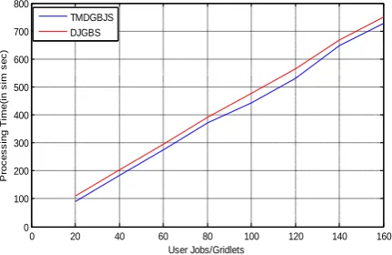
The Figure-4 given below represents the processing time of two algorithms for the Chunk_Size 10 with different user jobs of average MI 200 with deviation of 20%.
Observation:-2
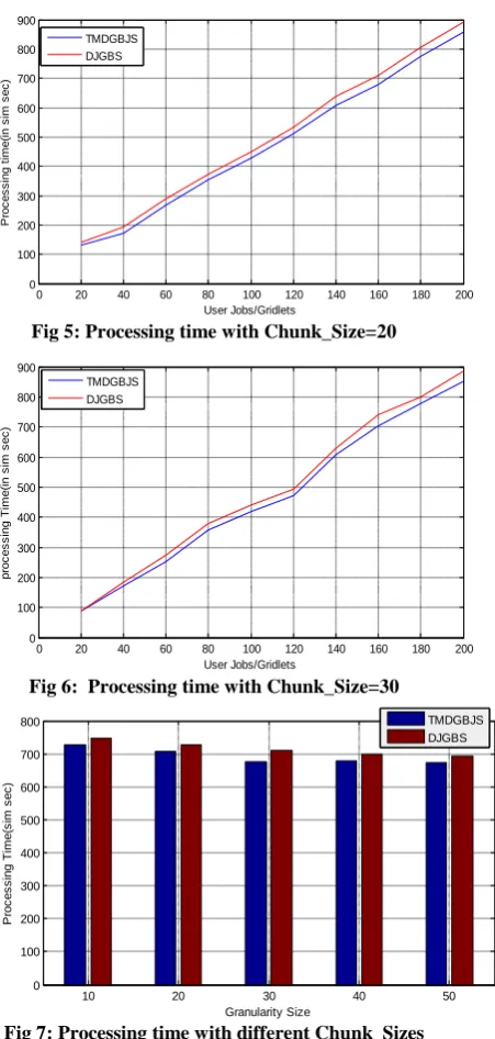
The Figure-5 corresponds to the processing time of two algorithms for the Chunk_Size 20 with different user jobs of average MI 200 with a deviation of 20%.
Observation:-3
The observation in Figure-6 signifies the processing time of two algorithms for the Chunk_Size 30 with different user jobs of average MI 200 with deviation of 20%.
Observation:-4
The Figure-7 illustrates the behavior of TMDGJS and DJGBS algorithms in terms of processing time for 160 Gridlets with different Chunk_Sizes.
Observation:-5
The Figure-8 depicts a sample of overhead time incurred by the two scheduling algorithms mentioned above for the Chunk_Size of 30 with different jobs of average MI 200 and a deviation of 20 %. The overhead time of 10 sim seconds is considered for all the resources.
[image:7.595.331.547.578.718.2]The performance gain of the proposed scheduling algorithm over DJGBS in simulation environment 1 is from 4.5% to18.3% in terms of processing time and from 4.2% to 8.4% in terms of overhead time.
Fig 4: Processing time with Chunk_Size=10
0 20 40 60 80 100 120 140 160 0
100 200 300 400 500 600 700 800
User Jobs/Gridlets
P
ro
c
e
s
s
in
g
Ti
m
e
(i
n
s
im
s
e
c
)
Fig 5: Processing time with Chunk_Size=20
[image:8.595.69.295.74.548.2]Fig 6: Processing time with Chunk_Size=30
[image:8.595.330.560.560.699.2]Fig 7: Processing time with different Chunk_Sizes
Fig 8: Overhead time with Chunk_Size=30
Simulation Environment: -2 (Jobs are created without any particular deviation percentage)
This simulation is intended to analyze the performance of the proposed scheduling algorithm and DJGBS in an environment where all Gridlets are created without any particular deviation percentage. Evaluation of processing time with respect to different number of Gridlets for Chunk_Sizes 10, 20, 30 are shown in observation 1, observation 2 and observation 3 respectively. Processing time for a fixed number of Gridlets without any particular deviation for different Chunk_Sizes is considered in observation 4. Similarly overhead time of both the algorithms is presented in observation 5.
Observation:-1
The Figure-9 given below depicts the processing time of two algorithms, where the jobs are created randomly without any specific deviation percentage with Chunk_Size of 10.
Observation:-2
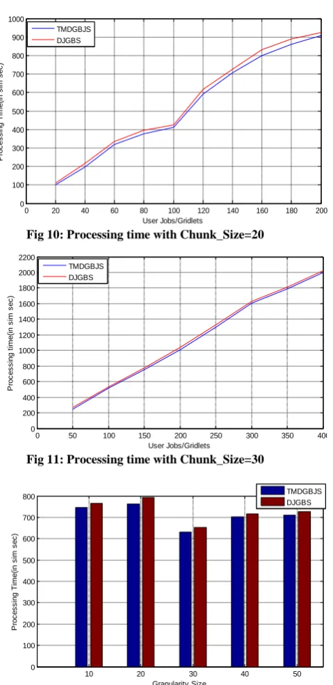
The Figure-10 given below depicts the processing time of two scheduling algorithms, with Chunk_Size of 20.
Observation:-3
Similarly, the Figure-11 illustrates the processing time of two algorithms for different number of randomly created user jobs within a Chunk_Size of 30.
Observation:-4
The Figure-12 depicts the processing time comparison of two algorithms for processing 160 numbers of Gridlets with different Chunk_Size.
Observation:-5
The figure-13 given below describes the overhead time of two algorithms for the different number of user jobs, where the jobs are created randomly without any particular deviation percentage within Chunk_Size of 30. The overhead time of 10 sim seconds is considered for all the resources. From the above observations in simulation environment 2, it can be seen that the performance enhancement in case of processing time is almost 4% to 22.48% and overhead time is 4.1% to 8.8%.
Simulation Environment:-3
This simulation takes different Chunk_Size for different resources. The Figure-14 shows the processing time of two scheduling algorithms for the different Gridlets. Here the Chunk_Sizes are taken from 5 to 50 with 5 unit of sim second increment for each of the resources starting from R1 to R10 as shown in table-1. The Performance enhancement in case of processing time is 3.6% to 14.1%.
Fig 9: Processing time with Chunk_Size=10
0 20 40 60 80 100 120 140 160 180 200 0
100 200 300 400 500 600 700 800 900
User Jobs/Gridlets
P
ro
c
e
s
s
in
g
t
im
e
(i
n
s
im
s
e
c
)
TMDGBJS DJGBS
0 20 40 60 80 100 120 140 160 180 200 0
100 200 300 400 500 600 700 800 900
User Jobs/Gridlets
p
ro
c
e
s
s
in
g
Ti
m
e
(i
n
s
im
s
e
c
)
TMDGBJS DJGBS
10 20 30 40 50
0 100 200 300 400 500 600 700 800
Granularity Size
P
ro
c
e
s
s
in
g
Ti
m
e
(s
im
s
e
c
)
TMDGBJS DJGBS
80 160 240 320 400 480 0
20 40 60 80 100
User Jobs/Gridlets
C
o
m
m
u
n
ic
a
ti
o
n
Ti
m
e
(s
im
s
e
c
)
TMDGBJS DJGBS
0 20 40 60 80 100 120 140 0
100 200 300 400 500 600 700 800
User Jobs/gridlets
P
ro
c
e
s
in
g
t
im
e
(s
im
s
e
c
)
[image:8.595.65.295.569.705.2]Fig 10: Processing time with Chunk_Size=20
Fig 11: Processing time with Chunk_Size=30
Fig 12. Processing time with different Chunk_Size
Fig 13: Communication time with Chunk_Size=30
Fig 14: Processing time with different Chunk_Size for different Resources
6.
CONCLUSION AND FUTURE WORK
Extensive simulation and the evaluation in varied grid environments are conducted to study and compare the behavior of the proposed TMDGJS and DJGBS. The simulation results have shown that the proposed scheduling algorithm is able to achieve the desired objectives in grid environment. The comparative study done through various observations shows that the proposed TMDGJS gives better performance than DJGBS in terms of processing time and overhead time. The complexity of the of the proposed dynamic job scheduling algorithm is О(nlogn) considering sorting of resources and Gridlets according to their MIPS and MI respectively, without which it will run in linear time. The overall performance improvement is up to 22.5% and 8.8% in terms of processing and overhead time respectively.
In future, this work can be extended to design a high performance cost-time scheduling for grid system to realize a real grid environment.
7.
REFERENCES
[1] Jeremy M. Norman (edited), From Gutenberg to the Internet: A Sourcebook on the History of Information Technology: 2005, pp. 870.
[2] L.Klienrock,“UCLA press release,” 1969, http://www.lk.cs.ucla.edu/LK/Bib/REPORT/ press.html
[3] I.Foster, and C. Kesselman, Globus: a metacomputing infrastructure toolkit, International Journal of High Performance Computing Applications, Vol. 2, pp. 115– 128, 1997.
[4] Ian Foster and Carl Kesselman, “The Grid: Blueprint for a New Computing Infrastructure,” Elsevier Inc., Singapore, Second Edition, 2004.
[5] Myer, Thomas, “Grid Computing: Conceptual Flyover for Developers”, May 2003 ,http://www-106.ibm.com/developerworks/library/gr-fly.html gridsrc.pdf
[6] M. Baker, R. Buyya, D. Laforenza, “Grids and Grid Technologies for Wide-area Distributed Computing”. SoftwarePractice & Experience, Vol 32, No. 15, 2002,pp. 1437 -1466
[7] D. Bernstein, M. Rodeh and I. Gertner, “On the Complexity of Scheduling Problems for Parallel/Pipelined Machines“, IEEE Transactions on Computers, vol. 38, p. 1308, 1998.
0 20 40 60 80 100 120 140 160 180 200 0 100 200 300 400 500 600 700 800 900 1000 User Jobs/Gridlets P ro c e s s in g Ti m e (i n s im s e c ) TMDGBJS DJGBS
0 50 100 150 200 250 300 350 400 0 200 400 600 800 1000 1200 1400 1600 1800 2000 2200 User Jobs/Gridlets P ro c e s s in g t im e (i n s im s e c ) TMDGBJS DJGBS
10 20 30 40 50
0 100 200 300 400 500 600 700 800 Granularity Size P ro c e s s in g Ti m e (i n s im s e c ) TMDGBJS DJGBS
80 160 240 320 400 480 0 10 20 30 40 50 60 70 80 90 100 User Jobs/Gridlets C o m m u n ic a ti o n Ti m e (i n s im s e c ) TMDGBJS DJGBS
0 50 100 150 200 250 300 350 400 200 400 600 800 1000 1200 1400 1600 1800 2000
User Jobs/ Gridlets
[image:9.595.326.561.80.220.2][8] S. You, H. Kim, D. Hwang, S. Kim, “Task Scheduling Algorithm in GRID Considering Heterogeneous Environment”, in The 2004 International Conference on Parallel and Distributed Processing Techniques and Applications (PDPTA'04), Monte Carlo Resort, Las Vegas, Nevada, USA, June 21 - 24, 2004, pp. 240-245.
[9] N. Muthuvelu, Junyan Liu, N.L.Soe, S.venugopal, A.Sulistio, and R.Buyya, “A dynamic job grouping-based scheduling for deploying applications with fine-grained tasks on global grids,” in Proc of Australasian workshop on grid computing, vol. 4, pp. 41–48, 2005. [10]Gray, J. (2003): Distributed Computing
Economics.Newsletter of the IEEE Task Force on Cluster Computing, 5(1), July/August
[11]Sarkar, V. (1989): Partitioning and Scheduling Parallel Programs for Execution on Multiprocessors, Cambridge, MIT Press.
[12]Gerasoulis, A. and Yang, T. (1992): A comparison of clustering heuristics for scheduling directed graphs on multiprocessors. Journal of Parallel and Distributed Computing, 16(4):276-291.
[13]Radulescu, A. and van Gemund, A. (1998): GLB: A Low-Cost Scheduling Algorithm for Distributed-Memory Architectures. Proc. of the Fifth International Conference on High Performance Computing(HiPC 98), Madras, India, pp. 294-301, IEEE Press
[14]James, H. A., Hawick, K. A. and Coddington, P. D. (1999): Scheduling Independent Tasks on Metacomputing Systems. Proc. of Parallel and Distributed Computing (PDCS ’99), Fort Lauderdale, USA
[15]Buyya, R., Date, S., Mizuno-Matsumoto, Y., Venugopal, S. and Abramson, D. (2004): Neuroscience Instrumentation and Distributed Analysis of Brain Activity Data: A Case for eScience on Global Grids. Journal of Concurrency and Computation: Practice and Experience
[16]Jeremy M. Norman (edited), From Gutenberg to the Internet: A Sourcebook on the History of Information Technology: 2005, pp. 870
[17]Ng Wai Keat, Ang Tan Fong, “Scheduling Framework For Bandwidth-Aware Job Grouping-Based Scheduling In Grid Computing”, Malaysian Journal of Computer Science, vol. 19, No. 2, pp. 117-126, 2006
[18]Quan Liu, Yeqing Liao, “Grouping-based Fine-grained Job Scheduling in Grid Computing”, IEEE First International Workshop on Educational technology And Computer Science, vol.1, pp. 556-559, 2009.
[19]M.K.Mishra, R. Sharma, V. K. Soni, B. R. Parida, R. K. Das(2010): A Memory-Aware Dynamic Job Scheduling Model in Grid Computing. International Conference on Computer Design and Applications, 2010 IEEE, vol.1-545.
[20]Schopf, J.: A General Architecture for Scheduling on the Grid. Submitted to special issue of JPDC on Grid Computing (2002).
[21]Buyya, R., Abramson, D., Giddy, J.: An Economy Driven Resource Management Architecture for Global Computational Power Grids. International Conference on Parallel and Distributed Processing Techniques and Applications (2000).
[22]Abraham A., Buyya R., Nath B.: Nature's Heuristics for Scheduling Jobs on Computational Grids. International Conference on Advanced Computing and Communications (2000).
[23]Abramson, D., Buyya, R., Giddy, J.: A Computational Economy for Grid Computing and its Implementation in the Nimrod-G Resource Broker. Future Generation Computer Systems Journal, Volume 18, Issue 8, Elsevier Science (2002) 1061-1074.