Volatility and Irish Exports

Munich Personal RePEc Archive

Volatility and Irish Exports

Cotter, John and Bredin, Don

University College Dublin

2005

Online at

https://mpra.ub.uni-muenchen.de/3522/

Volatility and Irish Exports

Don Bredin

University College Dublin∗

John Cotter

University College Dublin

April 2007

Abstract

We analyse the impact of volatilityper seon real exports for a small open economy concentrating on Irish trade with the UK and the US. An important element is that we take account of the time lag between the trade decision and the actual trade or payments taking place by using a flexible lag approach. Rather than adopt a single measure of risk we also adopt a spectrum of risk measures and detail varied size characteristics and statistical properties. We find that the ambiguous results found to date may be due to not taking account of the timing effect which varies substantially depending on which volatility measure is used.

Keywords: Exports, risk measurement, distributed lags

JEL Classification: C32, C51, F14, F31

∗_{Address for correspondence: Don Bredin, Centre for Financial Markets,}

Grad-uate School of Business, University College Dublin, Blackrock, Ireland; e-mail:

[email protected]; tel: + 00 353 1 716 8833; fax: + 00 353 1 283 5482. The authors

would like to thank Chris Baum, Mark Cassidy, G¨unter Edenharter, Liam Gallagher,

1

The international trade performance of a small open economy (SOE) plays a pivotal role in the performance of the economy. This is clearly the case for Ireland as the share of Irish merchandise exports in Gross Domestic Product (GDP) has grown dramatically in recent years (from 43% in 1979 to 94% in 2002), thus rendering the economy more open than before and more dependent on foreign markets.1

Hence, policies designed to enhance export performance are of increasing importance to national economic wel-fare. Good policy decisions are assisted by having relevant information on the factors that determine the level of exports and imports. In this paper, we examine the impact of volatilityper se on real Irish exports to the UK and the US using a two country imperfect substitutes model.2

As well as in-cluding real income and real foreign exchange, volatility of these underlying variables is also analysed by incorporating a spectrum of volatility proxies. The analysis of a small open economy’s export function is in contrast to the vast majority of the previous studies which focus on large economies with a small share of international trade relative to GDP. The issue of the sensitiv-ity to volatilsensitiv-ity considers both foreign exchange volatilsensitiv-ity as well as foreign income volatility. Moreover, in excess of 40% of Irish exports goes to the UK and US and these transactions dominate those of its trading partners within the auspices of the Euro currency union. Also the case of the Irish economy can provide unique insights into the effects of currency unions given it was part of a currency union with UK Sterling up until 1979.

There are a number of important advances in the current study to pro-vide insights on the mixed empirical findings for the impact of economic variables such as foreign exchange volatility on exports. Firstly, we adopt a comprehensive set of volatility measures and determine whether the use of a specific measure influences the empirics. These include recent advances in the time varying autoregressive heterosecasticity literature, APARCH, abso-lute volatility underpinned by the theory of power variation, and the model free log range estimate. This paper details their statistical properties in con-junction with their impact on real exports. The vast majority of previous studies report results for the influence of volatility on trade by focusing only on a single particular measure of foreign exchange volatility and in many cases have not accounted for the recent developments in time varying risk measurement. As well as exchange rate volatility, we expand the menu of

1

Ireland’s status as a SOE is clearly evident and especially its reliance on Non-Euro trade of over 60% of total trade dominated by its activities with the UK and US. In contrast, other economies in the European Union are not nearly as reliant on Non-Euro dominated trade.

2

volatility variables and determine the impact of foreign income uncertainty that is often overlooked but may well be crucial to a small open developing economy. The importance of foreign income volatility for trade has been highlighted (Franke (1991), Baum et al (2004), and Grier and Smallwood (2005). For instance, Franke (1991) views trade as an option for a firm that will be exercised if doing so is profitable. Thus as well as including income and foreign exchange in our exports model we include volatility of these underlying variables. This is consistent with Franke (1991), where foreign income volatility (rather than foreign exchange volatility) is viewed as a signal for greater profit opportunities. As well as addressing the impact of foreign exchange rate volatility and foreign income volatility, we also look at the interaction between the two following Baum et al (2004), and hence take account of any possible non-linear influences on exports that they may have.

Secondly, rather than looking at the empirical long-run relationship be-tween exports and a set of variables, we analyse the impact of volatilityper se adopting a flexible lag approach. Using a Poisson distributed lag struc-ture the model takes account of the lag between trade decisions and the time of the actual trade flow/payment. Thus our empirical results show the total effect of volatility as well as the distribution of the effect over time. A similar flexible lag approach has been adopted by both Baum et al (2004) and Klaassen (2004) for fully developed economies. However, in the current setting we are able to indicate the total effect as well as the time distribution effect for each of the complete set of foreign exchange and income volatility variables. A key issue is whether the various volatility measures are likely to have similar total and time distribution effects.

Finally, the data set studied is representative of a small open economy facing a high degree of uncertainty from external factors. Although a mem-ber of the European single currency, the majority of Irish exports are to non Euro zones with the US and the UK representing the most important markets.3

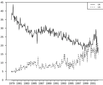
At the start of our sample in 1979 Irish exports to the US repre-sented just under 5% of total exports, while at the end of the sample it was close to 20%. In contrast, Irish exports to the UK have fallen from about 40% in 1979 to 20% in 2002. While the trend, in terms of the share of total Irish exports to the US and the UK, is moving in opposite directions, the combined importance remains extremely strong, i.e. over 40% of total Irish exports go to the US and the UK at both the beginning and the end of the sample.

3

The paper finds very strong evidence for the influence of volatility on a small open economy. We find that the foreign exchange volatility effect is consistently positive, indicating the dominance of exporters expectations of possible profitable opportunities from future cash flows associated with the export function. In contrast, the potential negative aspects of trade, the entry and exit costs, appear to be accounted for by negative effects for income volatility on trade. Moreover, positive non-linear effects for the interaction between foreign exchange and income volatility influence exports for a small open economy are reported. Importantly these findings occur in the face of volatility measures that differentiate considerably in their statistical properties according to the modelling process used. Moreover while the total effect of the foreign exchange and income volatility on exports is consistent across each of the various volatility measures, the timing effect is considerably different. This effect represents the time (in months) at which the maximum effect occurs and it varies significantly across our volatility measures. Overall we find that the ambiguous results found to date in the literature may be due to not taking account of the varying timing effect.

The remainder of the paper is organized as follows: Section 2 provides a survey of the theoretical and empirical literature. The methodological ap-proach with the operations of the adopted export model and the alternative volatility measures are discussed in detail in section 3. Section 4 includes a description of the data used and an analysis of the alternative volatility measures. Section 5 reports details of the model specification and the find-ings from our empirical model concentrating on the influence of volatility. Finally, section 6 concludes.

2

2.1 Theoretical models

Theoretically the modelling of exports allows for different impacts of volatility with no unanimity on direction and magnitude. To illustrate, De-mers (1991) assumed that exchange rate risk leads to lower production and trade due to price uncertainty implications for foreign demand. This ratio-nal is generally supported by policy makers (see EU Commission (1990)). Here, the effect of higher exchange rate volatility depends on the expected marginal utility of export income. Higher exchange rate risk reduces the ex-pected marginal utility of export revenues, and thus, risk averse producers reduce their output.

because they affect the real opportunities of the firm (De Grauwe, 1994). Assuming that firms make their production and export decisions once they have observed the exchange rate, higher exchange rate uncertainty may in-crease the average profit of the firm. For a profit-taking firm, a higher price due to an exchange rate change results in the firm enjoying higher profits per unit of output and so expands its output. Equivalently, in this anal-ysis, exporting represents an option. At a favourable exchange rate the firm exercises its option to export. The opposite happens for unfavourable movements. Since the value of options increase with the variability of the underlying asset, the firm is better off when exchange rate variability in-creases. Even assuming risk aversion, it remains possible that exchange rate volatility increases exports, provided that the increase in utility of the firm from the increase in the average profit, offsets the decline in utility of the risk averse firm due to the greater uncertainty of profits.

More specifically, Franke (1991) follows a real options approach and views trade as an option to be exercised by a firm. The author examines the decision making process of exporters under uncertainty in an intertem-poral multiperiod setting. The real options approach extends the possible factors included in modelling exports. In particular, any underlying variable has associated volatility giving rise to adding income and foreign exchange volatility to our export function. Here for example, the exchange rate is assumed to be mean reverting and there are costs to entering and exiting markets. Firms will exercise the option to enter a market if doing so is profitable. The profitability of the option depends on the present value of expected cash flows from exporting and on the present value of expected en-try and exist costs. A weaker (stronger) exchange rate increases (decreases) both the cash flow from exporting and entry and exit costs. The latter are assumed to be a concave function of the exchange rate. If volatility causes expected cash flows from exporting to grow faster than expected entry and exit costs, then the value of the option to export has increased and volatility and trade are positively related. This will be the case if cash flows are con-vex in the exchange rate. According to this scenario, increased volatility will result in firms entering the market sooner and exiting later and the number of trading firms will increase.

2.2 Empirical Evidence

The vast empirical evidence of the influence of exchange rate volatility on exports is also mixed. 4

Findings are dependent on models employed, sam-ple period analysed and countries examined (Bacchetta and van Wincoop, 2000). Furthermore there is no consistency in the measures of volatility used ranging from unconditional estimates such as standard deviation in the early literature to conditional ones such as GARCH estimates in more recent times (McKenzie, 1999). For instance, Koray and Lastrapes (1988) find evidence of a negative relationship between exchange rate volatility and trade using cointegration techniques involving US pairs. In contrast, Baum et al (2004) show evidence of a positive relationship between exchange rate volatility and trade using a poisson flexible lag structure, while Klaassen (2004) did not find evidence of any significant effect of exchange rate volatility on trade for G7 economies. Hedging through derivative products usually explains the lack of significance, although Wei (1999) finds a negative and statisti-cally significant effect for foreign exchange rate volatility on exports even after taking account of futures and options instruments to hedge risk. There is some evidence that views increased exchange rate volatility as a result of greater integration of world markets (see Rose, 2000). While Glick and Rose (2002), measuring exchange rate uncertainty using unconditional standard deviation, find that an increase (decrease) in exchange rate volatility result-ing from leavresult-ing (joinresult-ing) a currency union has a negative (positive) impact on trade statistics.

The majority of empirical studies estimate an export functions based on the following (see Arize, 1997):

xt=β0+β1y ∗

t +β2p ∗

xt+β3σs,t+ǫt (1)

where xt, yt∗, and pt, stand for real exports, foreign real income, and

relative prices, respectively (in logs), t represents time (in months), σs,t

stands for exchange rate volatility that captures exchange rate uncertainty andǫtrepresents the error term.5 Economic theory suggests that real income

levels of the trading partners for the domestic country and competitiveness measures affect the volume of exports positively and negatively respectively.

In addition to the mixed empirical results many alternative modelling approaches have been applied. Early empirical studies disregarded the issue of nonstationarity of macroeconomic time series and used classical regression analysis and are subject to the ”spurious regression” criticism (Granger and

4

See McKenzie (1999) for a review.

5

Relative prices,p∗

xt is defined as log(Pxt/Pt∗), where Pxt and Pt∗ are domestic and

Newbold, 1974). Studies also test for stationarity of the relevant time se-ries and employ cointegration techniques, e.g., Koray and Lastrapes (1989). Two recent studies take a different approach, Klaassen (2004) and Baum et al (2004). Rather than looking at the long-run relationship between the variables both papers analyse the impact of exchange rate volatility adopt-ing a flexible lag approach. In other words the model takes account of the lag between a trade decision and the time of the actual trade flow/payment. In both cases the empirical part of the studies use a Poisson lag structure in order to account for the possible extended effect. Klaassen focuses on US exports to other G7 countries for the period 1978 to 1996 and finds an insignificant effect in all cases.

Baum et al (2004) focuses on bilateral aggregate real exports between 1980 and 1998 for the following countries, US, Canada, Germany, UK, France, Italy, Japan, Finland, Netherlands, Norway, Spain, Sweden, and Switzerland. Baum et al (2004) also include foreign income volatility that is consistent with Franke (1991). We now view foreign income volatility as a signal for greater profit opportunities. As well as addressing the impact of foreign exchange rate volatility and foreign income volatility, they also look at the interaction between the two and hence take account of any possible non-linear relationship. Overall they find a significant impact of real income volatility on trade that varies in direction for the countries analysed.

Evidence on the impact of volatility on Irish trade statistics is relatively sparse.6

Thom and Walsh (2002), modelling overall Irish trade find no ev-idence that exchange rate regime changes impact Anglo-Irish trade from analysing time series and panel regressions in a case-study approach. The study argues that the unilateral move by Ireland to join the EMS is unique in that the devolvement did not disrupt trade. This was mainly due to the fact that both the UK and Ireland were both members of the then Euro-pean Economic Community (EEC). Also, Lothian and McCarthy (2000) find that foreign exchange volatility changes according to exchange rate systems and that volatility decreases upon joining a currency union vis-a-vis other systems.

3

3.1 Modelling Exports

As in Klaassen (2004) and Baum et al (2004) we adopt the flexible lag version of the Goldstein and Khan (1985) two country imperfect substitutes

6

model for bilateral trade between Ireland and the US and the UK in real terms. This allows for examining the decision making process of exporters under uncertainty for intertemporal multiperiod horizons. The variable of interest is real Irish exports, using Irish unit export value as our deflator.7

Irish exports to the UK and US are almost exclusively invoiced in UK Ster-ling and US Dollars respectively and we examine the logarithm of real Irish exports.8 _{The determinants of exports relate to the assumptions}

concern-ing export supply and demand. The determinants of demand are foreign income,y∗

t−l, and relative prices, p ∗

xt=log(Pxt/Pt∗), and both are stated in

foreign currency, while l is a lag representing the time delay between the purchase and delivery of the goods.9

q_td=qd(y∗

t−l, p ∗

xt) (2)

The determinants of the exports supply function only includes the rela-tive price of exports converted to domestic prices;

q_ts=qs(p∗

xt+st) (3)

where st is the log of the nominal exchange rate, measured as foreign

per unit of domestic currency. Given that decisions will be made based on the forecast of relative prices, both the conditional mean and the standard deviation ofp∗

xt+st are both included in the supply equation.

q_ts=qs(Et−_l[p ∗

xt+st], σs,t−_l[p ∗

xt+st]) (4)

forl is the lag to take account of potential time delay.

Goldstein and Khan (1985) assume that the export decision and actual exports and payments are not contemporaneous introducing a degree of un-certainty into the trade model. To incorporate this unun-certainty, the model is estimated with a flexible poisson lag structure. This allows for uncertainty between trading decisions and actual completion of trade and we examine how it impacts our variables in the export model. It makes the traders forward-looking and motivates the relevance of our income and exchange rate risk variables as potential determinants of trade (Klaassen, 2004). The

7

The Irish export sector is dualistic in make-up, with relatively smaller indigenous firms dominating the more low technology production sectors, while larger subsidiaries of foreign owned multinationals tend to dominate the more high technology sectors.

8

This practice has surprisingly continued even since the entry of Ireland to the Euro Zone and may influence our findings. For instance 68% of Irish exports to the UK are invoiced in UK Sterling, while 75% of Irish exports to the US are invoiced in US Dollars (Institute of International Trade of Ireland, 2005).

9

use of the lag structure allows the data to determine the dynamic specifica-tion of the timing effect. We allow each variable to have its own lag structure so thereby measure their maximum effect and illustrate their patterns. In addition, the process is extended following an options based approach by including volatility of the underlying variables. Furthermore there may be non-linear effects arising from a combination of income and foreign exchange volatility effects not directly measured in the variables alone (Baum et al, 2004). To incorporate this an interaction term of income and foreign ex-change volatility is introduced into the exporter’s supply function.10

Taking account of these extensions we can now re-write exports supply as:

qs_t =qs(Et−l[p ∗

xt+st], σs,t−l, σy,t−l, σs×y,t−l) (5)

where σs,t−l is real foreign exchange volatility, σy,t−l is real income

volatility both outlining direct effects, σs×y,t−l is the interaction term

in-corporating non-linear indirect responses of income and foreign exchange volatility on the supply function andlis the lag to take account of potential time delay. The interaction term, the product of foreign exchange and in-come volatility, may capture any possible non-linearities between exchange rate volatility and exports.

3.2 The Poisson Lag Approach

An important element is that we take account of the time lag between the trade decision and the actual trade taking place or payment taking place (Goldstein and Khan, 1985). Hence it is clearly not sufficient to account for only contemporaneous relationships between exports and our explanatory variables. Equating supply (equation 5) and demand (equation 2) leads to a function for real exports of the following form11

;

xt=β0+ Σ ∞

l=1[β1ly

∗

t−l+β2lEt−ls

r

t+β3lσs,t−l+β4lσy,t−l+β5lσs×y,t−l)] (6)

The β’s represent the sensitivities of exports to each of the variables in-cluded (real foreign income, real exchange rate, real foreign exchange rate volatility, real income volatility and the interaction term), e.g. β1lrepresents

the effect of foreign income on exports at the lag where the effect is largest. In order to model the impact using a flexible lag approach, we adopt a Pois-son lag structure (see Baum et al (2004) and Klaassen (2004)). Alternative,

10

A further motivation for including the interaction term is to take account of possible omitted variable bias. See Baum et al. (2004) for a discussion.

11

but more restrictive, approach’s include the geometric and the polynomial lag specification. For example the geometric approach implies that βl is

decreasing as the lag increases.12

The Poisson lag approach is derived from the Poisson probability distribution for each underlying variable;

βkl=βk.

(λk−1)l−1

(l−1)! exp[−(λk−1)] (7)

forλk≥1 andλis the lag at which the maximum effect occurs. One

im-portant advantage of the Poisson lag approach is the number of parameters to be estimated is minimized, 2k+ 1, wherekis the number of independent variables. As can be seen the parametersλ1, ...λk enter into the equation in

a non-linear fashion. In order to calculate the parameters λ1, ...λ_k, we use

the simulated annealing optimization technique (see, Goffe et al. 1994).13

Once the parameters,λ1, ...λk, have been obtained from the non-linear

opti-mization technique, the estimated coefficients,β1, ...β_k, are calculated using

OLS.

3.3 The Appropriate Volatility Measure

Our export model follows an options based approach. Here participation in export markets is based on evaluation of entry and exit costs using a real options approach to the decision making process. This real options approach suggests additional volatility variables affect medium term exports. The real options approach incorporates volatility of the economic variables under consideration thus including volatility of exchange rates and of income. In his study Franke (1991) finds a statistically significant positive relationship between exports and exchange rate volatility. The rational is that firms increase exports in response to increased volatility if the present value of expected cash flows from exports exceeds the sum of entry and exit costs. For instance, changes in the volatility of foreign income changes an exporting firm’s entry/exit cost ratio and therefore their export opportunities to that economy. Thus higher foreign income volatility may signal higher profit opportunities resulting in a change in exporters decision-making leading to increased exports.

Given the importance of volatility in our modelling process it is inter-esting to note that the literature relies on many different types of volatility

12

See Klaassen (2004) for a detailed discussion of the problems associated with geometric and polynomial lags in the current setting.

13

estimates (McKenzie, 1999). So for example, unlike exchange rates that are available contemporaneously exchange rate volatility is modelled ex-post. This has led to a major research agenda in trying to model financial volatil-ity through analysis of its distributional and dynamic characteristics. Major developments have been made in modelling the time-variation of volatility and its persistence and we incorporate a spectrum of these models. These include the autoregressive conditional heteroskedasticity (ARCH) related models and the more recent model-free aggregated based procedures under-pinned by the theory of power variation. In contrast, models that assume constant volatility are now generally ignored.14 _{Regardless of what approach}

is used, the key issue is to recognize that volatility is latently unobservable thereby requiring proxies. This gives rise to a modelling approach that could involve a spectrum of procedures and we estimate the export specification with a number of alternative risk measures to determine if volatility determi-nation impacts on inferences from the export model. Specifically we address the issue as to whether alternative volatility estimates are responsible for the inconclusive empirical evidence? By looking at a number of estimates we can ascertain the influence of volatility per se rather than be swayed by the conclusions from a single estimate. The paper focuses on four separate measures for foreign exchange and income respectively and when combined give rise to sixteen interaction terms. The foreign exchange and income measures necessarily diverge due to data availability, e.g. foreign exchange rates are available at relatively high frequencies such as daily intervals, while income estimates are only available at monthly frequencies.

The volatility measures come from different strands of the literature such as conditional measures where we apply a time-varying APARCH pro-cess that nests seven different parametric ARCH models (for a review see Bollerslev et al, 1994). Also, estimates underpinned by the theory of power variation such as realized volatility that requires aggregation from high to low frequency observations has been advocated with many illustrations for volatility modelling (see references in Andersen et al, 2003). Moreover, we examine the impact of other model free estimates using squared, absolute and range based estimates (see Ding and Granger, 1996; and Alizadeh et al, 2002).

First concentrating on the aggregated measures that are applied to the daily exchange rates, the most common approach suggests the use of ag-gregated squared exchange rate changes over a period, say for example, aggregating daily realisations to obtain monthly estimates instead of using

14

a single estimate from the monthly exchange rate changes (see Baum et al, 2004; Klaassen, 2004). This estimate is closely associated with the vari-ance. Merton (1980) illustrates the advantages in using relatively high fre-quency observations to obtain more precise low frefre-quency risk measures and early applications with monthly estimation cumulating daily observations are given in French et al. (1987). This paper also analyses aggregated abso-lute realisations that evolves from the same theoretical framework, realized power variation (see Barndorff-Nielsen and Shephard, 2003), as exchange rate changes have the stylized property of exhibiting fat-tails due to exces-sive large-scale movements and modelling with absolute realisations is more robust in the presence of this property (Davidian and Carroll, 1987). Also, more attractive time-series properties are documented for absolute realised volatility measures than their squared counterparts (Barndorff-Nielsen and Shephard, 2003).

Turning to the theoretical framework we begin by defining the price process that is underpinned by realised power variation. Volatility of this price process defined as integrated volatility is said to be unobservable. The framework incorporates the popularly used quadratic variation that details the use of aggregated squared realisations and absolute power variation us-ing aggregated absolute realisations. We analyse the price process that has rm,t =pt−pt−1/m as the compounded returns withm evenly spaced

obser-vations per month. Importantly, realised power variation that incorporates realised absolute variation, namely the sum of absolute realisations, Σ|rm|,

equate with integrated volatility, making volatility of the price process ob-servable.

We present power variations for both squared and absolute measures for monthly foreign exchange volatility. The practical implementation of the theory simplifies into constructing volatility estimators using aggregated absolute exchange rate changes and their variants for any month t withm daily intervals:

|rt|n= m

X

j=1

|rm,t+j/m|n (8)

where the power coefficients, n, can take on a range of values 0.5 < n <3 (see Barndorff-Nielsen and Shephard (2003)). Also, in terms of the commonly applied principle of quadratic variation using aggregated squared realisations exchange rate volatility is given as:

[r2_t]n=

m

X

j=1

where different power transformations are again underpinned by the the-oretical framework.

Moving to the standard modelling of time variation GARCH type pro-cesses have traditionally been applied (Kroner and Lastrapes, 1993; and Klaassen, 2004). A large number of specifications are available with for ex-ample, Kroner and Lastrapes (1993) using a GARCH-M process whereas Klaassen (2004) using a GARCH (1, 1) model. All these models have a common feature in modelling clustering of second moments. We use the Asymmetric Power ARCH (APARCH) to provide end of month income and foreign exchange rate volatility estimates. The model developed by Ding et al (1993) advantageously nests many extensions of the GARCH process. As well as encompassing three ARCH specifications (ARCH, Non-linear ARCH and Log-ARCH), two specifications of the GARCH model (using standard deviation and variance of returns), it also details two asymmetric models (both ARCH and GARCH versions). It is given by:

σ_td=α0+

p

X

i=1

αi(|ǫt−_i|+γ_iǫ_t−_i)d+

q

X

j=1

βjσdt−j (10)

for α0, αi, βj ≥ 0, αi+βj ≤ 1, −1 ≤ γi ≤ 1. The ǫt are the errors,

andσtis the conditional variance. Detailing the model, the process presents

volatility in the form of a Box-Cox transformation whose flexibility allows for different specifications of the residuals process associated with different GARCH models. As well as describing the time-variation in exchange rate changes, it also allows for the possibility of leverage effects, γi, by letting

the autoregressive term of the conditional volatility process be represented as asymmetric absolute residuals. Non-linear GARCH models are derived from different power coefficients, d. The model is fitted with a conditional student-t distribution thereby allowing for fat tails. The model adequately deals with second moment persistence documented for the underlying vari-ables.

In addition, the use of the log range defined as the first difference of the log of maximum and minimum prices is applied to foreign exchange data at monthly intervals. This simple estimate has been used widely in an ad hoc fashion in the literature and its time series properties are formally examined in Alizadeh et al (2002). They find that it is an efficient estimator with small measurement error and has further attractive time series properties by being approximately gaussian.

of proxying for unobservable volatility by using the observed absolute in-come changes and observed squared inin-come changes as measures of inin-come uncertainty. Ding and Granger (1996) show that these model free volatil-ity proxies adequately model the long term persistence property associated with financial data. The final income measure is the moving window ap-proach advocated by Thursby and Thursby (1987) to obtain adaptive risk measures. Here the moving window technique estimates income volatility for the US and the UK where the logarithm of real income is regressed on a quadratic trend for a six-month moving window. The root mean squared error of the regression represents the time-varying process for our volatility measure using relatively low frequency income data.

Taking income volatility and exchange rate volatility we produce an in-teraction term as a product of these variables. This allows us to not only examine the direct impact of the respective volatility estimates, but also assess whether there is an indirect influence of these volatilities through their interaction with each other. Following the real options approach both exchange rate and income volatility would both have a direct concurrent impact on exporters decision-making but there may also be an indirect in-fluence. To examine any combined effects of these separate dynamics, the interaction term between exchange rate and income volatility is included to help describe the exporters behaviour. This allows for the processing of information that is different from each volatility measure but combines both income and exchange rate volatility. Any indirect impact of the re-spective volatility measure is captured by this interaction variable and it may remove omitted variable bias by examining respective volatility mea-sures only. Thus exchange rate volatility could impact income volatility and vice versa. For each volatility measure we create an interaction term giving sixteen separate measures each labelled as a combination of the respective volatility measures, for example APARCH exchange rate volatility combined with Squared income changes. These combinations imply that the impact of the interaction term will not be constant, but will depend on the respective measures of volatility.

4

4.1 Data

by Ireland’s unit export value to obtain the real exports figure.15 _Given

real national income is only available at quarterly frequencies, monthly UK and US industrial production (constant prices) are used. Irish, UK and US export unit values are obtained at monthly intervals. The exchange rate data used in the study is daily UK Sterling per unit of euro and US Dollar per unit of euro adjusted from Irish Pounds in the pre-Euro period. The real exchange rate is calculated from the spot exchange rate and the ratio of domestic to foreign (US and UK) price indices.16 17

As shown in figure 1, Irish exports to the UK and US make up a sizable proportion of Irish exports. Although traditionally the UK was the impor-tant market for Irish exports, this has diminished in recent years. At the same time, exports to the US have grown steadily over the last number of years. Although moving in different directions, exports to both countries is sizable and is exposed to exchange rate movement pressures. Furthermore, Ireland has an unique relationship with the UK that has driven many of its economic policies. For example, in terms of foreign exchange, Ireland and the UK was part of a currency union between 1800 and 1979.18 _The

Irish pound - introduced in 1927 - was held in a 1 : 1 no-margins peg with Sterling until 1979 using an adhoc currency commission to maintain the ar-rangement. Prior to this there was no independent Irish pound since the Act of Union in 1800. The break from parity was due to Ireland’s decision to be a member of the European Monetary System (EMS) and the UK’s non-participation. The most important influences on the Irish decision to join the EMS decision were the perceived political benefits, the promise of ad-ditional EEC subsidies, and a desire to shift the currency’s nominal anchor from Sterling, then considered to be inflation prone, to the new ’zone of mon-etary stability’ based on the German mark (Economic and Social Research Institute, 1996). Overall foreign exchange volatility for the Irish economy has increased in real terms since 1979 compared to under the Sterling link (Lothian and McCarthy, 2000).

4.2 Volatility Measures

Using the respective volatility measures outlined we describe their sta-tistical properties and analyse similarities and divergences. We find a large

15

All remaining data is from Datastream.

16

Given the exchange rate is available at daily frequencies and the domestic and foreign prices are only available at monthly frequencies, we linearly interpolate the price series within the month. See Baum et al (2004) where a similar approach is adopted.

17

McKenzie (1999) highlights the distinction between real and nominal exchange rate volatility does not significantly affect the results.

18

divergence for the respective volatility estimates in terms of size, pattern and statistical properties. There also appears to be a high degree of per-sistence. For foreign exchange volatility the measures all exhibit a different scale as can be seen in figure 2, with a common large spike around the ERM crises in 1992/93. 19

Although time variation is captured by all measures, the APARCH measure is smoothest whereas the RANGE is noisiest. Irish exporters faced considerable variation in exchange rate volatility for both currencies across the sample period with a major increase evident during the 1992/93 currency crises that enveloped the EMS currencies. This was followed by a relatively tranquil period but volatility tended to increase in the early years of the Euro.

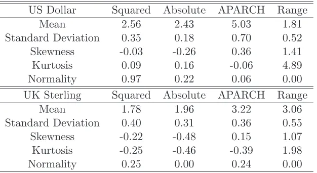
The summary statistics in table 1 outline the first four moments and the Jarque-Bera test for normality of foreign exchange volatility. The magnitude of moments varies considerably, with for example the mean spanning from 1.81 to 5.03 for the US whereas its standard deviation, the volatility of volatility measure exhibits a scale between 0.18 and 0.70. Non-gaussian features of excess skewness and excess kurtosis are documented in many cases, especially for the Range measures. The Range is prone to fat-tails with positive skewness.

Similar departures are indicated for the respective income volatility mea-sures. Notwithstanding the divergences, the result of the US expansionary policy increases all volatility measures in the early 80’s and there has also been a common increase in income volatility for the UK in 2002. Fur-thermore, all the measures exhibit excess skewness and kurtosis in table 2 and are non-normal. The excess skewness and kurtosis is strongest for the squared measure whereas APARCH exhibits a platykurtotic bunching of re-alisations. Diverging patterns of the respective measures also occurs with the squared and absolute measures noisy relative to APARCH and moving window volatility. The shape plots in figure 3 indicate that all the volatility measures are non-normal with excess positive skewness. Also all measures exhibit very fat upper tails. Whilst generally strong persistence is shown for all foreign exchange volatility measures in figure 4, it disappears after six months for US squared volatility.

Turning to the income volatility estimates we examine their relationship with each other and find that the APARCH estimate involves the lowest

19

linkages and a strong relationship exists between squared and absolute mea-sures for both UK and US. The extent of the relationships between respective foreign exchange rate volatility measures is shown in the scatter plots of fig-ure 5 for the UK and clearly indicates divergences. For instance, linkages between the squared and other measures is high, but in contrast the range is not strongly related to the other measures with correlations of less than 0.4 in both US and UK cases.

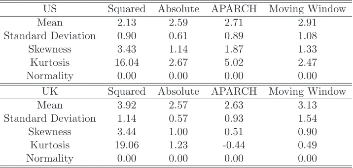
Given the respective divergences for income and foreign exchange volatil-ity measures, and the interaction term being defined as a combination of these, it is no surprise to see similar conclusions for the respective inter-actions in table 3. For instance, the standard deviation extends between 0.57 and 1.54 with very different patterns emerging across the interaction terms. Whilst this is especially so for those estimates involving Squared measures, all measures exhibit excess skewness and kurtosis and deviate from normality. Finally the varying strength of the relationships of the respective interaction terms incorporating the APARCH foreign exchange volatility measures are present with reasonably similar patterns. Thus for both US and UK exhibit strong linkages between Absolute and Squared measures with correlations in excess of 0.86 in comparison to the other rela-tively weak relationships. Overall the respective volatility measures diverge strongly in terms of size, pattern and statistical properties. These find-ings are consistent for both UK and US volatility measures. Given these discrepencies these inputs are now used to model Ireland’s export function with it largest trading partners to determine their respective influence on the economy’s exports.

5

5.1 Model Specification

The export model is run with forecasted volatility using the poisson lag structure for 16 combinations for each country pair.20

Our study includes

20

four separate foreign exchange risk measures, as well as four separate in-come volatility measures. We combine each of the foreign inin-come measures with the separate foreign exchange volatility measures, giving 16 possible combinations, to which we augment the interaction term, e.g. the specifi-cation may include Squared foreign exchange volatility, APARCH foreign income volatility and the interaction term,Squared-APARCH. As has been discussed an important element is that we take account of the time lag be-tween the trade decision and the actual trade taking place or payment taking place.21

The stochastic optimization process of simulating annealing is ap-plied to our function in order to obtain the global maximum. As has been discussed previously, this approach is adopted due to the difficulty associated with obtaining the global maximum. The algorithm is re-run with different starting values and a different seed for the random number generator and in all cases the optima were found to be identical. Consistent with Baum et al (2004) we allow for a maximum of 30 lags, however we do not restrict the final four variables to have the same lag; real foreign exchange, real foreign exchange volatility, real foreign income volatility, and the interaction term. Our unrestricted approach is taken to fully capture the exposure of exports from a small open economy from foreign exchange and income volatility.

The lag structure and the parameter coefficients of the models are of interest. The former details the optimal lag of exporters with respect to variables impacting their export decision whereas the latter shows the impact of economic variables such as income volatility on the export decision. Given that the volatility measures exhibit considerable deviations it is interesting to determine their respective impacts on the estimation of the lag structures for the export model. This would possibly help to explain the diverging results in the literature for volatility and trade.

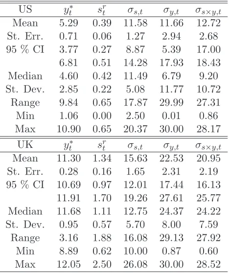
Summary statistics of the different lag structures affecting the variables in the export model in terms of mean and variance are given in table 4 for each country. Also a plot of the lag distribution for income and real exchange rates and associated volatility for exports to the UK and US is given in Figure 6. Unlike previous studies we do not assume an identical lag structure for each of our volatility terms. Different maximal lags are evident across the explanatory variables including foreign exchange and associated volatility. For instance the strongest lag effect occurs for real exchange rates having a mean of 0.39 compared to 11.58 for real exchange rate volatility for the US. However consistency in the lag structures for specific variables is generally evident, with the US generally having lower mean lags than the UK. In particular, exports to the US is generally affected quicker by economic wealth and foreign exchange activity compared to the impact of those variables for

21

the UK.22 _{Also for the specific lag structures, the mean of the maximal}

lag for real income is much higher for the UK (11.30) than the US (5.29). The latter is in line with the fast decline predicted by Goldstein and Khan (1985). The relatively large income lag for the case of exports to the UK is similar to Klaassen (2004) analysing developed economies although the study assumed the mean and variance of the lag structure to be equivalent.

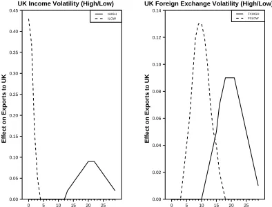
Turning to the volatility lag structures, both US and UK average real for-eign exchange volatility measures have their maximal impact after a number of lags of just less than a year. Also, the 95% interval estimate for real forex volatility is between 8.87 and 14.28 with a median of 11.49 months for the US. However, there is a fair degree of dispersion according to each model with a range of lags of over a year for both countries indicating that the largest effects vary according to different foreign exchange volatility mea-sures. This can be seen in figure 7, which plots the distribution associated with the highest and lowest lag effect. The pattern of lag weights suggest a hump shape in line with Klaassen (2004) and Baum et al (2004). The maximal effect for income volatility (figure 8) also varies with a median of 6.79 for the US and 24.37 for the UK with standard errors around 2 suggest-ing that exports respond slowly to economic activity. Again there is a large dispersion between minimum and maximum lags that present the strongest effects for income volatility measures on Irish exports. Finally the average lag of the interaction term is over a year and shows a large level of dispersion across the different models. Overall, the different volatility measures result in large variations in the export model’s lag structure and emphasise the importance of accounting for the respective lag structures.

Comparing the lag structures of the exchange rate and income variables the findings support previous studies (for example, Goldstein and Khan (1985) and Klaassen (2004)) in supporting a larger delay in the impact of foreign exchange over income variables.

5.2 Volatility and Exports

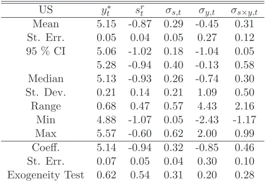
Estimated parameters for the export models are given in table 5 sum-marising the results for the 16 models for each country pair. We also report the point coefficients as well as standard errors for one of the regression combinations.23

A number of summary estimates of the 16 models are given

22

The results here could also reflect the distinct nature of the structure of exports to the US and the UK. In particular exports to the US are dominated by information computer and technology (ICT) and medical devices, while the UK figures are heavily influenced by the food and drink sector.

23

including the mean coefficient, and the minimum and maximum coefficients, and measures of dispersion of the coefficients including the standard devia-tion and range. The diagnostics indicate well specified models in all cases, e.g. highR2_{and no evidence of edogeneity of regressors.}24 _{Very strong}

pos-itive real income effects are reported with all t-statistics significant. These large positive coefficients are associated with a low dispersion of estimates with a minimum of 4.88 for the US and a maximum of 5.57. The point es-timates for the US follow the same pattern as the UK. The negative effects of real foreign exchange are consistent with theory and in line with previous studies that measure their variables in foreign currency. Also, the impact of foreign exchange is reasonably constant with very little dispersion indicated for the country pair parameters. The parameters are consistent across the country pairs with coefficients of similar magnitude.

The main empirical issue of the paper examines the impact of volatility on exports using the small open Irish economy as a case study and is now outlined. As discussed, many studies have investigated the influence of real exchange rate volatility with very contradictory findings. For Ireland, real exchange rate volatility has a positive impact on trade and statistically sig-nificant regardless of the foreign exchange volatility measure applied. On average a 1% increase in respective foreign exchange volatility leads to an increase in exports to the US and the UK by 0.29% and 0.17%. Further-more, the specific model (squared approach) indicated that a 1% increase in foreign exchange volatility leads to an increase in exports to the US and the UK by 0.32% and 0.11% respectively. Although there is some varia-tion (in particular for exports to the US), the relavaria-tionship is positive in all cases. The results imply that exporters treat an increase in real foreign ex-change volatility to the US and UK as a positive situation to exploit profit opportunities associated with the positive expected cash flow dominating the entry and exit costs of exporting. Exporters then decide to exercise their option to trade resulting in increased trade flows being determined by increased foreign exchange volatility. The positive effect of real foreign exchange volatility supports the findings of Franke (1991) and Baum et al (2004). The consistency of the finding occurs given the backdrop of diverg-ing magnitude and statistical properties documented across the volatility measures (see table 1).

Dispersion of the impact of foreign exchange volatility measures does occur, indicating that the choice of volatility proxies matter. For instance, the smallest effect (minimum value = 0.05) occurs for the Range volatility measure in the US equation but is still statistically positive with a t-statistic

24

of 2.85. In contrast, the largest effect (maximum value = 0.62) occurs for the APARCH measure for the US with a t-statistic of 7.57. The results also suggest that exports to the US are considerably more sensitive to the respective foreign exchange volatility measures relative to UK exports.

International evidence regarding the impact of income volatility on ex-port flows is sparse. Baum et al (2004) find that income volatility is sig-nificant in only a quarter of their cases and claim that the sign of the sta-tistically important parameters is ambiguous with nearly as many negative influences as positive influences being recorded. We find stronger results in adopting the real options approach and the respective influence of income volatility with significant influences being found in all but three of the thirty two cases, one being negative and two being positive. Our findings are in line with Grier and Smallwood (2005) who use a GARCH specification for a mixture of developing and developed economies. Overall foreign income volatility is primarily a negative determinant of Irish exports to the US in 11 models and to the UK in 15 models. For instance on average a 1% in-crease in foreign income volatility reduces Irish exports to the US and the UK by 0.45% and 0.81% respectively. The finding suggests that the nega-tive impact of exit and entry costs driven by the export decision dominates the cash flow benefits associated with greater levels of income volatility and results in reduced trade as exporters do not exercise their option to trade in these circumstances. Furthermore, the negative coefficients recorded in the remaining models dominate the positive findings as evidenced by the mean statistic and their associated confidence interval in table 5. The average impacts are reasonably similar for the US and UK, with the latter dominat-ing. However, the range of impact is relatively large for the different models applied, with values of 1.39 for the UK and 4.43 for the US.

6

The paper analyses the impact of real foreign exchange and income volatility on Irish exports to the UK and the US. The majority of the lit-erature in this area has focused on exports from fully developed economies and may well have led to the inconclusive empirical evidence to date. This issue has been highlighted by Bacchetta and Wincoop (2000) and Baum et al (2004) who suggest that data selection issues may be driving the mixed results. This study reverses the analysis by focusing on a small open econ-omy with a very high dependency on trade and potentially high levels of volatility affecting the factors driving exports.

Of interest is the effect of foreign exchange and income volatility on Irish exports to the UK and the US over the period studied, 1979-2002. Although Ireland is a member of the Euro, the remaining foreign exchange volatility effects may be substantial as a large percentage of Irish exports are to the UK and the US. This was especially the case for the Sterling rate, which previously had a currency union with the Irish currency pre 1979, and also was part of the EMS between 1990 and 1992. In terms of the effect of foreign exchange volatility, we find that there is a consistently positive effect on Irish exports to the UK and the US. In contrast we find a negative impact of income volatility on exports, a result which is consistent with Franke (1991). If the exporting decision is viewed as an option, as suggested by Franke (1991), then our income volatility result highlights that the costs of entry dominate the increased cash flows associated with the export decision, resulting in lower exports. Finally, we also test the impact of the interaction between foreign exchange rate and income volatility, and find a positive effect in the majority of cases. This illustrates an indirect effect of foreign exchange and income volatility on the export function.

References

Alizadeh, S., M. W. Brandt, and F. X. Diebold (2002), “Range Based Es-timation of Stochastic Volatility Models“, Journal of Finance, 57, pp. 1047-1092.

Andersen, T. G., T. Bollerslev, and F. X. Diebold (2003), “Parametric and nonparametric measurement of volatility“, In Y. Ait-Sahalia and L. P. Hansen (Eds.): Handbook of Financial Econometrics, Amsterdam: North Holland.

Arize, A.C. (1997), ”Conditional Exchange Rate Volatility and the Volume of Foreign Trade: Evidence from Seven Industrialized Countries”,

South-ern Economic Journal 64, pp. 235-254.

Bacchetta, P, and E. van Wincoop. (2000), “Does Exchange Rate Stability Increase Trade and Welfare?`‘, American Economic Review 90, pp. 1093-1109.

Barndorff-Nielsen, O. E. and N. Shephard (2003), “Realised power variation and stochastic volatility“,Bernoulli 9, pp. 243-265.

Baum, C. F., M. Caglayan, and N. Ozkan (2004), “Nonlinear Effects of Exchange Rate Volatility on the Volume of Bilateral Exports“,Journal of

Applied Econometrics Vol. 19, pp. 1-23.

Bollerselv, T., R.F. Engle and D.B. Nelson (1994), “ARCH Model“, PP. 2959-3038, In R.F. Engle and D.C. McFadden (eds.)Handbook of

Econo-metrics, Amsterdam: Elsevier Science.

Central Bank & Financial Services Authority of Ireland, Quarterly Bulletin, Spring 2004.

Davidian, M., & Carroll, R. J. (1987), “Variance Function Estimation“,

Journal of the American Statistical Association, 82, pp. 1079-1091.

Demers, M. (1991), ”Investment Under Uncertainty, Irreversibility, and the Arrival of Information over Time”,Review of Economic Studies, Vol. 58, pp. 333-350.

De Grauwe, P. (1994),The Economics of Monetary Integration, Oxford Uni-versity Press, Oxford.

Ding, Z., C. W. J. Granger and R. F. Engle (1993), “A Long Memory Prop-erty of Stock Market Returns and A New Model“, Journal of Empirical

Finance, Vol. 1, pp. 83-106.

Economic & Social Research Institute (1996), ”Economic Implications for Ireland of EMU” , Policy Research Series, Paper No. 28.

EU Commission (1990), ”One Market, One Money,”European Economy, 44.

Franke, G. (1991), ”Exchange Rate Volatility and International Trading Strategy”,Journal of International Money and Finance, Vol. 10, pp. 292-307.

French, K.R., G.W. Schwert and R.F. Stambaugh (1987), ”Expected Stock Returns and Volatility”, Journal of Financial Economics, 19, pp. 3-29.

Glick, R and A. K. Rose (2002), ”Does a currency union affect trade? The time-series evidence”, European Economic Review 46, pp. 1125 - 1151.

Goffe, W.L., G.D. Ferrier, J. Rogers (1994), ”Global Optimization of Sta-tistical Functions with Simulated Annealing”, Journal of Econometrics, Vol. 60, pp.65-100.

Goldstein, M. and M.S. Khan (1978), ”The Supply and Demand for Ex-ports: A Simultaneous Equation Approach”, The Review of Economics

and Statistics, Vol. 60, pp. 275-286.

Granger, C. W. J., and Z. C. Ding (1995), ”Some Properties of Absolute Returns, An Alternative Measure of Risk”, Annales d’Economie et de

Statistique, Vol. 40, pp. 67-91.

Grier, K., and A. Smallwood (2005), ”Uncertainty and Export Performance: Evidence from 18 Countries”,University of Oklahoma Working Paper.

Institute of International Trade of Ireland (2005), Export Ireland Survey

2005 - International Trade, Finance and Credit Management.

Klaassen, F. (2004), ”Why is it so Difficult to Find an Effect of Exchange Rate Risk on Trade?”, Journal of International Money and Finance, 23, pp. 817-839.

Kroner, K.F. and W.D. Lastrapes (1993), ”The Impact of Exchange Rate Volatility on International Trade: Reduced Form Estimates Using the GARCH-in-Mean Model,” Journal of International Money and Finance, 12, pp. 298-318.

Lastrapes, W.D. and F. Koray (1990), ”Real Exchange Rate Volatility and US Multilateral Trade Flows”, The Journal of Macroeconomics, Vol. 12, pp. 341-362.

McKenzie, M. D. (1999), ”The Impact of Exchange Rate Volatility on In-ternational Trade Flows”,Journal of Economic Surveys 13, pp. 71-106.

Merton, R.C. (1980), ”On Estimating the Expected Return on the Market: An Exploratory Investigation”, Journal of Financial Economics, 8, pp. 323-361.

Rose, A.K. (2000), ”One money, one market: Estimating the effect of com-mon currencies on trade”.Economic Policy 20 April, pp. 7-45.

Thom, R., and Walsh, B. (2002), ”The effect of a common currency on trade: Ireland before and after the Sterling link”.European Economic Review 46, pp. 1111-1123.

Thursby, J, and M. Thursby (1987), ”Bilateral Trade Flows, the Linder Hypothesis, and Exchange Risk”,The Review of Economics and Statistics, Vol. 69, pp. 488-495.

Viaene, J.-M. and C.G. de Vries (1992), ”International Trade and Exchange Rate Volatility,” European Economic Review, 36, pp. 1311-1321.

Wei, S.J. (1999), ”Currency Heding and Goods Trade”,European Economics

Figure 1: Exports to the UK and US as Percentage of Total Irish Exports

1979 1981 1983 1985 1987 1989 1991 1993 1995 1997 1999 2001 0 5 10 15 20 25 30 35 40 45 UK US

Figure 2: Monthly Foreign Exchange Volatility Plots

US

US Dollar Time

Squared

1982 1986 1990 1994 1998 2002

1.6 3.2 US US Dollar Time Absolute

1982 1986 1990 1994 1998 2002

1.9 2.7 US US Dollar Time APARCH

1982 1986 1990 1994 1998 2002

4.0 6.0 US US Dollar Time Range

1982 1986 1990 1994 1998 2002

1.5 3.5 UK UK Sterling Time Squared

1982 1986 1990 1994 1998 2002

0.8 2.4 UK UK Sterling Time Absolute

1982 1986 1990 1994 1998 2002

1.2 2.0 UK UK Sterling Time APARCH

1982 1986 1990 1994 1998 2002

2.6 4.2 UK UK Sterling Time Range

1982 1986 1990 1994 1998 2002

2.0

Figure 3: Monthly Income Volatility Shape Plots for US

Squared

Probability density

0.5 1.0 1.5

0

1

2

3

Quantiles of Standard Normal

Squared

-3 -2 -1 0 1 2 3

0.4

0.8

1.2

Absolute

Probability density

0.2 0.4 0.6 0.8 1.0 1.2

0

1

2

3

Quantiles of Standard Normal

Absolute

-3 -2 -1 0 1 2 3

0.4

0.8

APARCH

Probability density

0.2 0.4 0.6 0.8 1.0 1.2 1.4

0

1

2

3

Quantiles of Standard Normal

APARCH

-3 -2 -1 0 1 2 3

0.4

0.8

1.2

Moving Window

Probability density

0.0 0.5 1.0 1.5

0.0

1.0

2.0

Quantiles of Standard Normal

Moving Window

-3 -2 -1 0 1 2 3

0.2

0.6

1.0

Figure 4: Monthly Income Volatility Persistence Plots

US

No. Lags

ACF - Squared

2 4 6 8 10 12

0.1 0.2 0.3 0.4 US No. Lags

ACF - Absolute

2 4 6 8 10 12

0.2

0.4

0.6

US

No. Lags

ACF - APARCH

2 4 6 8 10 12

0.3

0.5

0.7

US

No. Lags

ACF - Moving Window

2 4 6 8 10 12

0.2 0.4 0.6 0.8 UK No. Lags

ACF - Squared

2 4 6 8 10 12

-0.1

0.1

0.3

UK

No. Lags

ACF - Absolute

2 4 6 8 10 12

0.20

0.35

UK

No. Lags

ACF - APARCH

2 4 6 8 10 12

0.80

0.90

UK

No. Lags

ACF - Moving Window

2 4 6 8 10 12

0.3

0.5

0.7

Figure 5: Monthly UK Foreign Exchange Volatility Scatter Plots

Squared

1.0 1.5 2.0 2.5

1 2 3 4 5

0.5 1.0 1.5 2.0 2.5

1.0 1.5 2.0 2.5

Absolute

APARCH

2.1 2.6 3.1 3.6 4.1

0.5 1.0 1.5 2.0 2.5 1 2 3 4 5

2.1 2.6 3.1 3.6 4.1

Range

Figure 6: Poisson Lag Distribution on Real Foreign Income and Foreign Exchange

UK Income & Foreign Exchange

Effect on Exports to UK

0 5 10 15 20 25 0.00

0.05 0.10 0.15 0.20 0.25 0.30 0.35

UKY UKFX

US Income & Foreign Exchange

Effect on Exports to US

0 5 10 15 20 25 0.0

0.1 0.2 0.3 0.4 0.5 0.6 0.7

Figure 7: Poisson Lag Distribution on Real Foreign Income and Foreign Exchange Volatility for UK

UK Income Volatility (High/Low)

Effect on Exports to UK

0 5 10 15 20 25 0.00

0.05 0.10 0.15 0.20 0.25 0.30 0.35 0.40 0.45

IHIGH ILOW

UK Foreign Exchange Volatility (High/Low)

Effect on Exports to UK

0 5 10 15 20 25 0.00

0.02 0.04 0.06 0.08 0.10 0.12 0.14

FXHIGH FXLOW

Figure 8: Poisson Lag Distribution on Real Foreign Income and Foreign Exchange Volatility for US

US Income Volatility (High/Low)

Effect on Exports to US

0 5 10 15 20 25 0.00

0.25 0.50 0.75 1.00

IHIGH ILOW

US Foreign Exchange Volatility (High/Low)

Effect on Exports to US

0 5 10 15 20 25 0.00

0.05 0.10 0.15 0.20 0.25 0.30

Table 1: Summary Statistics of Foreign Exchange Volatility

US Dollar Squared Absolute APARCH Range

Mean 2.56 2.43 5.03 1.81

Standard Deviation 0.35 0.18 0.70 0.52

Skewness -0.03 -0.26 0.36 1.41

Kurtosis 0.09 0.16 -0.06 4.89

Normality 0.97 0.22 0.06 0.00

UK Sterling Squared Absolute APARCH Range

Mean 1.78 1.96 3.22 3.06

Standard Deviation 0.40 0.31 0.36 0.55

Skewness -0.22 -0.48 0.15 1.07

Kurtosis -0.25 -0.46 -0.39 1.98

Normality 0.25 0.00 0.24 0.00

Table 2: Summary Statistics of Income Volatility

US Income Squared Absolute APARCH Moving Window

Mean 0.43 0.52 0.54 0.59

Standard Deviation 0.18 0.11 0.16 0.22

Skewness 3.35 1.25 1.85 0.99

Kurtosis 14.25 2.53 4.25 1.06

Normality 0.00 0.00 0.00 0.00

UK Income Squared Absolute APARCH Moving Window

Mean 1.22 0.80 0.82 0.97

Standard Deviation 0.33 0.15 0.25 0.46

Skewness 4.99 1.54 0.20 1.07

Kurtosis 34.67 3.95 -0.85 1.31

Normality 0.00 0.00 0.00 0.00

Notes: The volatility estimates are defined in the text. The figures for normality refer to p-values for the Bera-Jarque test.

Table 3: Summary Statistics of the Interaction Term (APARCH)

US Squared Absolute APARCH Moving Window

Mean 2.13 2.59 2.71 2.91

Standard Deviation 0.90 0.61 0.89 1.08

Skewness 3.43 1.14 1.87 1.33

Kurtosis 16.04 2.67 5.02 2.47

Normality 0.00 0.00 0.00 0.00

UK Squared Absolute APARCH Moving Window

Mean 3.92 2.57 2.63 3.13

Standard Deviation 1.14 0.57 0.93 1.54

Skewness 3.44 1.00 0.51 0.90

Kurtosis 19.06 1.23 -0.44 0.49

Normality 0.00 0.00 0.00 0.00

Table 4: Summary Statistics of the Poisson Lag Structure

US y∗

t srt σs,t σy,t σs×y,t

Mean 5.29 0.39 11.58 11.66 12.72

St. Err. 0.71 0.06 1.27 2.94 2.68

95 % CI 3.77 0.27 8.87 5.39 17.00

6.81 0.51 14.28 17.93 18.43

Median 4.60 0.42 11.49 6.79 9.20

St. Dev. 2.85 0.22 5.08 11.77 10.72

Range 9.84 0.65 17.87 29.99 27.31

Min 1.06 0.00 2.50 0.01 0.86

Max 10.90 0.65 20.37 30.00 28.17

UK y∗

t srt σs,t σy,t σs×y,t

Mean 11.30 1.34 15.63 22.53 20.95

St. Err. 0.28 0.16 1.65 2.31 2.19

95 % CI 10.69 0.97 12.01 17.44 16.13

11.91 1.70 19.26 27.61 25.77

Median 11.68 1.11 12.75 24.37 24.22

St. Dev. 0.95 0.57 5.70 8.00 7.59

Range 3.16 1.88 16.08 29.13 27.92

Min 8.89 0.62 10.00 0.87 0.60

Max 12.05 2.50 26.08 30.00 28.52

Note: y∗

t refers to real income, srt is real foreign exchange rate, σs,t is real

foreign exchange volatility, σy,t is real income volatility, and σs×y,t is the

Table 5: Summary Statistics of the Estimates of the Model

US y∗

t srt σs,t σy,t σs×y,t

Mean 5.15 -0.87 0.29 -0.45 0.31

St. Err. 0.05 0.04 0.05 0.27 0.12

95 % CI 5.06 -1.02 0.18 -1.04 0.05

5.28 -0.94 0.40 -0.13 0.58

Median 5.13 -0.93 0.26 -0.74 0.30

St. Dev. 0.21 0.14 0.21 1.09 0.50

Range 0.68 0.47 0.57 4.43 2.16

Min 4.88 -1.07 0.05 -2.43 -1.17

Max 5.57 -0.60 0.62 2.00 0.99

Coeff. 5.14 -0.94 0.32 -0.85 0.46

St. Err. 0.07 0.05 0.04 0.30 0.10

Exogeneity Test 0.62 0.54 0.31 0.20 0.28

R2

= 0.97, Standard Error = 0.16

UK y∗

t srt σs,t σy,t σs×y,t

Mean 2.72 -1.07 0.17 -0.81 -0.01

St. Err. 0.11 0.04 0.02 0.13 0.05

95 % CI 2.49 -1.15 0.12 -1.10 -0.10

2.96 -0.98 0.22 -0.52 0.09

Median 2.54 -1.10 0.15 -0.99 0.04

St. Dev. 0.37 0.14 0.08 0.46 0.16

Range 1.19 0.48 0.24 1.39 0.46

Min 2.25 -1.35 0.10 -1.26 -0.27

Max 3.44 -0.87 0.34 0.12 0.20

Coeff. 3.11 -1.14 0.11 -1.07 0.06

St. Err. 0.21 0.13 0.05 0.22 0.05

Exogeneity Test 0.51 0.49 0.19 0.21 0.19

R2

= 0.92, Standard Error = 0.16

Note: y∗

t refers to real income, srt is real foreign exchange rate, σs,t is real

foreign exchange volatility, σy,t is real income volatility, and σs×y,t is the