Least squares estimation of a shift in linear processes

Munich Personal RePEc Archive

Least squares estimation of a shift in

linear processes

Bai, Jushan

Massachusetts Institute of Technology

16 February 1993

Online at

https://mpra.ub.uni-muenchen.de/32878/

Least Squares Estimation of a Shift in Linear

Processes

by

Jushan Bai

Massachusetts Institute of Technology

Feburary 16, 1993

Mailing Address:

Department of Economics

E52-274B

Massachusetts Institute of Technology

Cambridge, MA 02139

U.S.A.

Abstract

This paper considers a mean shift with an unknown shift point in a linear process

and estimates the unknown shift point (change point) by the method of least squares.

Pre-shift and post-shift means are estimated concurrently with the change point. The

consistency and the rate of convergence for the estimated change point are established.

The asymptotic distribution for the change point estimator is obtained when the

mag-nitude of shift is small. It is shown that serial correlation affects the variance of the

change point estimator via the sum of the coefficients (impulses) of the linear process.

When the underlying process is an ARMA, a mean shift causes overestimation of its

order. A simple procedure is suggested to mitigate the bias in order estimation.

Keywords. Mean shift; linear processes; change point; rate of convergence; order

1.

Introduction and notations

The problem of a mean shift with an unknown shift point in an independent and

identically distributed sequence has received considerable attention in the literature.

Sen and Srivastava (1975a,1975b), Hawkins (1977), Worsley (1979, 1986), James,

James, and Siegmund (1987), and Srivastava and Worsley (1986) proposed tests for

testing a shift in a sequence of normal means. Hinkley (1970), Bhattacharya (1987),

Yao (1987), and many others considered the estimation of the shift point in a sequence

of independent variables. For serially correlated data, Picard (1985) estimated a shift

in a Gaussian autoregressive process with a known order. These authors considered

maximum likelihood estimation (MLE).

In this paper, we apply the least squares method (LS) to the estimation of a shift

point. Unlike the MLE, the LS method does not need to specify the underlying error

distribution function and is computationally simple. The least squares procedure

also allows a broader specification of correlation structure in the data than MLE can

typically permit. In particular, we assume that observations are drawn from a linear

process of martingale differences, rendering ARMA processes as special cases. When

the underlying process is assumed to have an ARMA representation, the orders of the

process is not assumed to be known. This is important because of the following two

reasons. First, in practice, orders of an ARMA process are rarely known and have

to be estimated. Second, order determination via the AIC and BIC criteria tends

to overestimate the order of an ARMA process if a shift exists, as was reported by

MacNeill and Duong (1982). In this paper, a simple procedure is suggested to alleviate

the bias caused by a mean shift when estimating the orders.

The model considered in this paper is as follows:

Yt=µ(t) +Xt (t=· · ·,−2,−1,0,1,2,· · ·) (1)

given by

Xt =

∞

X j=0

ajεt−j =a(B)εt (2)

with a(B) =P∞

j=0ajBj, Blεt=εt−l (l ≥0), andεt being white noise.

We consider the simple case that µ(t) only takes two different values, µ1 before

time k0 and µ2 after time k0. That is,

µ(t) = (

µ1 if t_≤k0

µ2 if t > k0

where µ1, µ2, and k0 are unknown and k0 is the change point.

The problem is to estimate µ1, µ2, and k0 givenT observations Y1, Y2,_{· · ·}, YT. We assume that k0 = [T τ] for some τ _∈ (0,1), where [_·] is the integer-valued function. When Xt has an ARMA representation, we may also want to estimate its orders as

well as its coefficients.

The least squares (LS) estimation of a shift is not new. Hawkins (1986) examined

the LS method for a shift in an i.i.d. sequence. He proved that T1/2−δ(ˆτ ₋τ)_→0 in probability for any δ >0, where ˆτ is the LS estimator of τ (defined below). Hawkin’s

rate of convergence is improved in this paper despite serial correlations in observations.

We shall show that T(ˆτ ₋τ) = Op(1). We also show how serial correlation in data affects the variance of the change point estimator. In particular, we find that , when

Xt is an ARMA process given by Ψ(B)Xt= Θ(B)εt, the variance of the change point

estimator is smaller than that of an i.i.d. sequence with a shift if _|Θ(1)Ψ(1)−1_|<1.

Throughout this paper, we assume:

(A) the εt are i.i.d. with mean zero and variance σ2, or

(A′_{) the ε}

t are martingale differences satisfying: E(εt|Ft−1) = 0, Eε2t = σ2,

n−1Pn

t=1E(ε2t|Ft−1) → σ2, and there exists a δ > 0 such that suptE|ǫt|2+δ < ∞, where _Ft is the σ-field generated by εs, s≤t.

We shall focus on the estimation of the change point. Once the change point is

estimated, µ1 and µ2 can be estimated by using the estimated pre-change and post

follows:

ˆ

k = argmin_k 

min µ1,µ2

 

 k X t=1

(Yt−µ1)2+ T X t=k+1

(Yt−µ2)2  

 

. (3)

Thus the shift point is estimated by minimizing the sum of squares of residuals among

all possible sample splits. Statistical properties of this estimator will be examined in

later sections.

We denote the mean of the first k observations by ¯Yk and the mean of the last

T ₋k observations by ¯Y∗

k. If the shift point is k, then ¯Yk and ¯Yk∗ are the usual least squares estimators of µ1 and µ2, respectively. The corresponding sum of squares of

residuals is

S_k2 = k X t=1

(Yt−Y¯k)2+ T X t=k+1

(Yt−Y¯k∗)2.

Thus ˆk= argmin_k(S2

k) and the LS estimators forµ1 andµ2 are ˆµ1 = ¯Yˆk and ˆµ2 = ¯Y_kˆ∗,

respectively. Next, write ¯Y = ¯YT, which is the overall mean of the given data. Since

for each k (1_≤k _≤T ₋1), T X t=1

(Yt−Y¯)2 =Sk2 +Vk2

where

Vk=

k(T ₋k)

T

!1/2

( ¯Y_k∗₋Y¯k), (4)

it follows that

ˆ

k = argmin_k(S_k2) = argmax_k(V_k2) = argmax_k|Vk|.

As will be seen, the statistical properties of the change point estimator are obtained

by studying the behavior of Vk and the argmax functional.

Denote the LS residuals by ˆXt, which is defined as

ˆ

Xt=Yt−µ1ˆ −(ˆµ2−µ1ˆ )I(t >ˆk),

where I(_·) is the indicator function. We shall call ˆXt the generalized residuals in view of the presence of a change point estimator. If Xt is an ARMA process, then

experiments show that the order estimation based on ˆXtyields almost identical results

as those based on Xt, thus providing a practical solution to the problem reported by

MacNeill and Duong (1984). This two step procedure for estimating the parameters

of the model is much simpler than MLE from the computation point of view.

Denote ˆτ = ˆk/T. We shall establish the consistency, the rate of convergence,

and the limiting distribution of ˆτ in the following several sections. We shall first,

however, generalize the H´ajek and R´enyi inequality to serially correlated variables.

This inequality is important to our results.

2.

A generalization of the H´

ajek and R´

enyi

in-equality

Let ε1, ε2,_{· · ·}, be a sequence of martingale differences with Eε2

i = σ2, and {ck} be a decreasing positive sequence of constants. H´ajek and R´enyi (1955) proved that

P r max

m≤k≤nck| k X i=1

εi|> α !

≤ σ

2

α2



mc2_m+ n X i=m+1

c2_i



. (5)

This inequality was initially stated in terms of i.i.d. random variables and was later

generalized to martingales by Birnbaum and Marshall (1961). We now generalize this

inequality to serially correlated variables. Let Xt be given by (2). We assume:

(B) P∞

j=0j|aj|<∞.

This condition is satisfied for stationary ARMA processes. Under assumptions (A or

A′_{) and (B), the generalized H´ajek and R´enyi inequality takes the following form:}

P r max

m≤k≤nck| k X i=1

Xi|> α !

≤Aσ 2

α2



mc2_m+ n X i=m+1

c2_i



, (6)

where A < _∞ is a constant only depending on the a′

js. The proof is given in the appendix. For ck = 1/k, because P∞k=mk−2 =O(m−1), we have

P r sup

k≥m 1

k|

k X i=1

Xi|> α !

for some A1 <∞. The weak law of large numbers is an immediate consequence of the

above inequality. Next consider the case ck = 1/

√

k and m= 1. By inequality (6),

P r sup

1≤k≤n 1 √ k| k X i=1

Xi|> α !

≤Aσ 2 α2 n X k=1 1 k ≤

Clogn α2

for some C >0. This implies

sup

1≤k≤n 1 √ k k X i=1 Xi

=Op(qlogn) (8)

Furthermore, the following invariance principle holds for Xt under assumptions (A or

A′_{) and (B) (see Hall and Heyde 1980, Theorem 5.5, p. 141-146),}

T−1/2 [T s]

X t=1

Xt⇒(

∞

X j=0

aj)σB(s) (9)

where B(s) is a standard Brownian motion on [0,1].

3.

The consistency of

τ

ˆ

The proof of consistency is almost standard. Recall how we prove, in general, the

con-sistency of an estimator obtained by maximizing an objective function. We need to

argue that the objective function converges uniformly in probability to a

nonstochas-tic function of parameters and that the nonstochasnonstochas-tic function has a unique global

maximum. The objective function in our problem is _|Vk| (k = 1,2,· · ·, T −1). How-ever, we will be able to work with Vk (without the absolute sign). This is because

the expected values of Vk (k = 1,2,· · ·, T −1) do not change signs. We shall prove that the expected value of Vk has a unique maximum at k0 and that (Vk −EVk) is uniformly small in k for large T.

First notice that

|Vk| − |Vk0| ≤ |Vk−EVk|+|Vk0 −EVk0|+|EVk| − |EVk0| (10)

≤ 2 sup k |

Vk−EVk| !

For the sake of simplicity, we shall assume that T τ itself is an integer and is equal to

k0. Writed=k/T and τ =k0/T. We next show that_|EVk| achieves its maximum at

k =k0 by showing that

|EVk0| − |EVk| ≥Cτ|λ(d−τ)| (12)

for some Cτ >0, where λ=µ2−µ1 is the magnitude of shift. We need only consider the case k_≤k0 because of symmetry. We assume without loss of generality thatλ >0 (otherwise consider the series ₋Yt). Then

EVk=

1₋τ

1₋d{d(1−d)}

1/2_{λ >0 fork}

≤k0. (13)

In particular, EVk0 ={τ(1−τ)}1/2λ. It follows that

|EVk0| − |EVk|=λ

{τ(1₋τ)_}1/2_{− {}d(1₋d)_}1/2(1₋τ)(1₋d)−1

=λ(1₋τ) 

 τ

1₋τ

1/2

− ₁ d −d

!1/2 .

Multiplying and dividing the above expression by [τ /(1₋τ)]1/2 _{+ [d/(1−d)]}1/2_{, we}

obtain

|EVk0| − |EVk|=λ

τ ₋d

1₋d



 τ

1₋τ

1/2

+ d

1₋d

!1/2 

−1

(14)

≥ 1₂λ(τ ₋d) τ

1₋τ

−1/2

.

This proves (12) for Cτ = [τ /(1−τ)]−1/2/2. By (11), (12), and |Vˆ_k| − |Vk0| ≥ 0, we obtain immediately (replacing d by ˆτ = ˆk/T),

|τˆ₋τ_{| ≤}2C_τ−1λ−1sup k |

Vk−EVk|.

From (4),

Vk−EVk =T− 1

2(k/T)(T −k)−1/2 T X t=k+1

Xt−T− 1

2(1−k/T)k−1/2 k X t=1

Xt,

hence

|Vk−EVk| ≤T− 1 2



(T −k)−1/2 T X t=k+1

Xt

+k−1/2

k X t=1 Xt 

It follows from (8) that the above is T−1/2_O

p(logT) uniformly in k. Therefore

|τˆ₋τ_|= (T−1/2λ−1)Op(logT), (16)

establishing the consistency. Notice that λ is kept on the right hand side in order to

illustrate how the rate depends on the magnitude of change. In addition, this allows us

to incorporate the case that λ varies with the sample sizeT. In fact, we will examine

specifically the case of a small change in the sense that λ = λT → 0. When λ is a fixed constant, (16) implies that T1/2−δ_{(ˆτ −τ)→}p _{0 for any δ > 0, giving rise to the} result of Hawkins (1986) for i.i.d. errors. This result is improved in the next section.

4.

The rate of convergence

We shall establish the stronger result:

ˆ

τ₋τ =Op 1

T λ2

. (17)

To this end, choose a δ > 0 such that τ _∈ (δ,1₋δ). Since ˆk/T is consistent for τ, for every ǫ >0,P r(ˆk/T _6∈(δ,1₋δ))< ǫ whenT is large. Thus we now only need to examine the behavior of Vk over those k for which T δ≤k≤T(1−δ). To prove (17), we shall prove that P r(_|τˆ₋τ_|> M(T λ2₎−1_{) is small when T and M are large. For}

every M >0, define DT,M ={k; T δ≤k ≤T(1−δ),|k−k0|> M λ−2}. Then

P r_|τˆ₋τ_|> M(T λ2)−1

≤P r(ˆτ _6∈(δ,1₋δ)) +P r_|τˆ₋τ_|> M(T λ2)−1,τˆ_∈(δ,1₋δ)

≤ǫ+P r sup k∈DT ,M

|Vk| ≥ |Vk0| !

.

Because _|x_{| ≥ |}y_| implies eitherx₋y_≥0 and x+y _≥0 or x₋y_≤0 and x+y _≤0, we have

P r sup

k∈DT ,M

|Vk| ≥ |Vk0| !

≤P r sup k∈DT ,M

Vk−Vk0 ≥0 !

+P r sup k∈DT ,M

Vk+Vk0 ≤0 !

def

We next argue that P1 and P2 are small when T and M are large. Define b(k) =

{(k/T)(1₋k/T)_}1/2 _{(k = 1,2, ...T). The following fact will be useful:}

0_≤b(k)_≤1, _|b(k0)₋b(k)_{| ≤}B_|k0₋k_|/T for some B >0 (18)

Now consider P2.

P2 = P r sup

k∈DT ,M

{EVk0 −Vk0 −(Vk−EVk)} ≥EVk0 +EVk !

≤ P 2 sup k∈DT ,M

|Vk−EVk| ≥EVk0 !

since EVk >0

≤ P r



2 sup T δ≤k≤T(1−δ)

b(k) 1

T ₋k

T X t=k+1

Xt− 1 k k X t=1 Xt

≥EVk0 



≤ P r



2 sup k≤T(1−δ)

1

T ₋k

T X t=k+1

Xt

≥ 1₂EVk0 

+P r 2 sup k≥T δ

1 k k X t=1 Xt ≥ 1 2EVk0

!

.

Because EVk0 = {τ(1−τ)}1/2λ, inequality (7) implies that each of the two terms above converges to zero as T tends to infinity.

The argument forP1 is more delicate. Note that

P1 =P r sup

k∈DT ,M

{Vk−EVk−(Vk0 −EVk0)} ≥EVk0 −EVk !

.

However,

Vk−EVk−(Vk0 −EVk0)

=b(k) 

 1

T ₋k

T X t=k+1

Xt− 1 k k X t=1 Xt 

−b(k0) 

 1

T ₋k0

T X t=k0+1

Xt− 1 k0 k0 X t=1 Xt   = 

b(k0) 1

k0

k0 X t=1

Xt−b(k) 1 k k X t=1 Xt  +  

b(k)

T ₋k

T X t=k+1

Xt−

b(k0)

T ₋k0

T X t=k0+1

Xt 



def

= G(k) +H(k). (19)

Since (EVk0 −EVk)≥Cτλ(k0−k)/T by (12), we have

P1 ≤ P r sup

k∈DT ,M

|G(k)_|> 1

2λ

|k0₋k_|

T C

!

+P r sup k∈DT ,M

|H(k)_|> 1

2λ

|k0₋k_|

T C

!

def

We now prove that P1,1 is small if T and M are large. Again because of symmetry,

we consider only the case of k _≤k0 and k _∈DT,M. More precisely, we consider those

k′_{s such that T δ ≤k ≤ T τ −M λ}−2_{. By adding and subtracting terms, G(k) can be}

written as:

G(k) = b(k0) k₋k0

kk0

k0 X t=1

Xt+{b(k0)−b(k)}

1

k

k X t=1

Xt+b(k0)

1

k

k0 X t=k

Xt (20)

By (18) and k _≥T δ, we have

|G(k)_{| ≤} k0 −k

T δk0 k0 X t=1 Xt

+Bk0−k T 1 T δ k X t=1 Xt

+k0−k

T δ

1

k0₋k

k0 X t=k+1

Xt . (21)

It follows that

P1,1 ≤ P r

1

T τ|

T τ X t=1

Xt|> 1 2δλC

!

+ P r sup

1≤k≤T 1

T|

k X t=1

Xt|> 1 2δλCB

−1

!

+ P r sup k≤T τ−M λ−2

1

T τ ₋k|

T τ X t=k

Xt|> 1 2δλC ! ≤ A 2σ δCτ 2 1

T λ2 +A

2Bσ

δC

2 1

T λ2 +

4A1 δ2_C2_M

by inequality (6) and (7). The last three terms are negligible when T andM are large.

The proof for P1,2 is similar.

5.

The limiting distribution

In this section, we aim to derive the asymptotic distribution of ˆτ when the sample

size increases to infinity. The limiting distribution provides a way for constructing

confidence intervals for the change point. The limiting distribution also provides some

qualitative aspects on how the estimated change point is related to other parameters

in the model. We now assume that λ depends on T and it diminishes as T increases.

When λ is a constant not depending on T, the results of Hinkely (1971a, 1971b) for

distribution of the innovations εt and also on λ in quite an intricate way. Thus

confidence intervals can not be easily constructed. In addition, whenλis large (relative

to the variance of the innovations), the estimation of the change point is quite precise.

Thus it might be more important to be able to construct confidence intervals for small

changes. Furthermore, a confidence interval based on the limiting distribution for

small λ is expected to cover the corresponding interval when λ is actually large and

thus can always be used as a more conservative confidence interval even if λ is large.

We shall useV(k) andVk interchangeably in this section. Now denoteλ byλT. If

λT is not too small in the sense that T1/2λT/logT → ∞, then the estimator ˆτ is still consistent, as can be seen from (16). The consistency in turn leads to (17).

Let us now assume that, for some 0< α <1/2

(C) λT →0,T1/2−αλT → ∞.

This assumption is sufficient for ˆτ to be consistent and is used by Picard (1985). Also

note that λT ≫T−1/2. From (17), we have ˆτ −τ =Op(T−1λ−T2), or equivalently,

ˆ

k₋k0 =Op(λ−_T2). (22)

Notice

ˆ

k = argmax_k(V2

k) = argmaxkT

V2

k −Vk02

.

Given the rate of convergence in (22), to study the limiting distribution, we only need

to examine the behavior of T(V2

k −Vk02) for those k in the neighborhood of k0 such that k = [k0+vλ−_T2], wherev varies in an arbitrary bounded interval. We shall obtain some weak convergence result forT(V2

k −Vk02) and then apply the continuous mapping theorem for the argmax functional. The idea is similar to that of Picard (1985) and

Yao (1987). To this end, connect by linear segments the points (k, V2

k −Vk02) ∈

R2_{, (k= 1,2,· · ·, T −1) and define:}

ΛT(v) =T nV([k0+vλ_T−2])2₋V(k0)2o.

We will find the limiting process of ΛT on _|v_{| ≤} M for every given M > 0. Let

Theorem 1. Under assumptions (A), (B), and (C), then for every M < _∞, ΛT(v)

converges weakly in C[₋M, M] to

Λ(v) = 2

a(1)σW(v)₋ 1 2|v|

(23)

and

T λ_T2(ˆτ ₋τ)_→d a(1)2σ2argmax_v

W(v)₋1 2|v|

(24)

where a(1) = P∞

j=0aj and W(v) is a two-sided Brownian motion on R. A two-sided

Brownian motion W(v) is defined as W(v) = W1(₋v) for v <0 and W(v) = W2(v)

for v _≥ 0 where Wi(v) (i = 1,2) are two independent Brownian motions defined on the non-negative half real line.

As a consequence of Theorem 1, we have

Theorem 2. When Xt is a stationary ARMA(p,q) process such that

Xt =ρ1Xt−1+· · ·+ρpXt−p+εt+θ1εt−1+· · ·+θqεt−q,

then

T λ_T2(ˆτ₋τ)_→d 1 +θ1+· · ·+θq 1₋ρ1_{− · · · −}ρp

!2

σ2argmax_v

W(v)₋ 1 2|v|

. (25)

A few comments are in order. First, ifa(1) = 0, Theorem 1 implies thatT λ2

T(ˆτ−

τ) _→p 0, a degenerate limiting distribution. Thus the convergence rate will be faster than T λ2

T. A simple example of a(1) = 0 is given by the first order moving average process Xt = εt−εt−1. Second, in Theorem 2, when θ1 =· · ·θq = 0 and ρ1 = · · ·=

ρp = 0, the right hand side of (25) gives the limiting distribution corresponding to the

case of i.i.d. normal variables with a shift in mean and the result is consistent with that

of Bhttacharya (1987) and Yao (1987). Third, (25) agrees with the result of Picard

(1985) for a pure autoregressive process (θ1 =_{· · ·}θq = 0) under normality assumption with maximum likelihood estimation. Thus it is reasonable to expect that (25) is

also the limiting distribution of the maximum likelihood estimator for ARMA model

find that the effect of serial correlation in Xt can be beneficial or detrimental to the

precision of the change point estimates depending on whether

1 +θ1+_{· · ·}+θq 1₋ρ1_{− · · · −}ρp

<1.

For example, in the ARMA(1,1) case (stationary and invertible), a negative ρ1 and a

negative θ1 should help us in locating the change point. On the other hand, when ρ1

is near the (positive) unit root, the change point estimator has a large variance since

(1₋ρ)−1 _{can be very large. These qualitative results are all confirmed by Monte Carlo}

simulations.

Proof of Theorem 1.We only consider the case of v _≤0 because of symmetry. Define the set KT(M) = {k; k is the integer part of k0 +vλ−T2 for all |v| ≤ M}. Notice

T(V_k2₋V_k20) = 2T Vk0(Vk−Vk0) +T(Vk−Vk0)

2

= 2T (EVk0)(Vk−Vk0) + 2T(Vk0 −EVk0)(Vk−Vk0) +T(Vk−Vk0)2. (26)

Let us first prove that the last two terms on the right are negligible onKT(M). Since

T1/2_(V

k0 −EVk0) is stochastically bounded due to (15), it is enough to show that

T1/2_(V

k−Vk0) is negligible on KT(M). Because,

T1/2_|Vk−Vk0| ≤ T

1/2

|Vk−EVk−Vk0 +EVk0|+T

1/2

|EVk−EVk0|

= T1/2_|G(k) +H(k)_|+T1/2_|EVk−EVk0|, (27)

whereG(k) andH(k) are defined in (19), it suffices to show that each of the two terms

on the right converges to zero uniformly on KT(M). It is clear that whenk ∈KT(M), there exists aδ >0 such thatk _≥T δ. Thus the upper bound forG(k) given in (21) is valid. This bound consists of three terms. Consider the first term of (21) multiplied

by T1/2_,

T1/2k0−k T δk0 k0 X t=1 Xt ≤ M

δτ T λ2

T 1

T1/2

k0 X t=1 Xt = 1

T λ2

T

uniformly for k_∈KT(M). The second term of (21) can be treated similarly. Consider the third term of (21) multiplied by T1/2_,

T1/2 1 T δ k0 X t=k+1

Xt = 1

T1/2_λ

T λT k0 X t=k+1

Xt (29)

Because λT

Pk0 t=k+1Xt

=Op(1) uniformly onKT(M) by the invariance principle (the number of elements in KT(M) is no larger than 2M λ−T2), (29) converges to zero in probability uniformly. Similarly, we can show that T1/2_{H(k) is negligible on K}

T(M). Next consider the second term of (27). Notice that

0_≤T1/2(EVk0 −EVk) = T

1/2 _b(k0)λ

T −b(k)

T ₋k0

T ₋k λT

!

≤ T1/2_{b(k0)₋b(k)_}λT +T1/2b(k)|

k0₋k_| T ₋k λT.

From (18) and k _∈ KT(M), we can easily show that T1/2(EVk0 −EVk) is bounded by C(T1/2_λ

T)−1 for some C > 0, which converges to zero. We now prove that for

k = [k0+vλ−_T2]

2T (EVk0)(Vk−Vk0) = 2{τ(1−τ)}1/2T λT{V(k0+vλT−2)−V(k0)} (30)

has the stated limiting distribution. For the sake of simplicity, we shall assume that

k0+vλ2

T and thus vλ2T are integers. By (19) we have

T λT(Vk−Vk0) = T λT{G(k) +H(k)} −T λT(EVk0 −EVk). (31)

As in proving (28), we can easily show that the first two terms in (20) multiplied by

T λT are op(1) uniformly on KT(M). However the product ofT λT and the third term

of (20) does not vanish as T increases and can be written as:

T λT b(k0) 1

k

k0 X t=k+1

Xt=b(k0)

T k



 λT

|v|λ−2

T

X t=0

Xk0−t 

 

for k = k0 +vλ−_T2. By the invariance principle of (9), (λT P

|v|λ−2

T

Moreover, b(k0) = {τ(1−τ)}1/2 andT /k →τ−1 fork ∈KT(M), thereforeT λTG(k0+ vλ−_T2) converges weakly to

τ−1_{τ(1₋τ)_}1/2a(1)σW1(₋v).

Similarly, we can prove that

T λTH(k0+vλT−2) = op(1) +b(k0)

T

T ₋k

  λT

|v|λ−2

T

X t=0

Xk0−t   .

As b(k0)T /(T ₋k)_→(1₋τ)−1_{τ(1−τ)}1/2_{, we have}

T λT{G(k0+vλ−T2) +H(k0+vλ−T2)} ⇒(τ−1 + (1−τ)−1){τ(1−τ)}1/2a(1)σW1(−v) =_{τ(1₋τ)_}−1/2a(1)σW1(₋v). (32)

From (14),

T λT(EVk0 −EVk) = T λ2T

τ ₋d

1₋d



 τ

1₋τ

1/2

+ d

1₋d

!1/2 

−1

→ |v_|{τ(1₋τ)_}−1/2/2 (33)

since d = k/T _→ τ uniformly on KT(M) and T λ2T(τ −d) = −v = |v|. Combining (30) to (33), we obtain for v _≤0,

ΛT(v)_⇒2

a(1)σW1(₋v)₋1 2|v|

.

Similarly, working with the case for v >0, we find that

ΛT(v)_⇒2

a(1)σW2(v)₋ 1 2|v|

,

wherea(1)σW2(v) is the limiting process ofλT Pkt=k0+1Xt =λT P vλ2

T

t=1 Xk0+t. It remains to show that W1(_·) and W2(_·) are independent. From (A.1) in the appendix,

λT k0 X t=k+1

Xt =λT k0 X t=k+1

a(1)εt−λTXk0∗ +λTXk∗

but supk∈KT(M)λT|X

∗

byεt witht≤k0. Similar arguments show thatW2(·) is determined byεt witht > k0.

Thus W1 and W2 are determined by non-overlapping sequences of _{εt} and hence

W1 and W2 are independent. This finishes the proof of (23). To prove (24), define

Cmax[₋M, M] to be the subset of C[₋M, M] such that each function has a unique maximum. It is straightforward to show that the argmaxfunctional is continuous on

the set Cmax[₋M, M]. This together with (22) permits us to invoke the continuous mapping theorem, which implies

T λ2_T(ˆτ₋τ)_→d argmax_vΛ(v).

For a rigorous treatment of the continuous mapping theorem for argmax functionals,

see Kim and Pollard (1990). Since bW(v) =d W(b2_{v) for every b ∈ R, a change in}

variable leads to argmax_vΛ(v) =d a(1)2_σ2_argmax

s(W(s)− |s|/2), which is (24). The proof of Theorem 1 is now complete.

Given the rate of convergence of ˆτ in Section 4, it is an easy matter to obtain the

limiting distributions of ˆµ1 and ˆµ2. Recall that ˆµ1 = ¯Yˆ_k and ˆµ2 = ¯Y∗

ˆ

k.

Proposition 1.

T1/2(ˆµ1₋µ1)_→d N(0, τ−1a(1)2σ2), (34)

T1/2(ˆµ2₋µ2)_→d N(0,(1₋τ)−1a(1)2σ2). (35)

Thus the limiting distributions are the same as if k0 is known. The proof is given in

the appendix.

6.

Monte Carlo simulation

In this section, we assess through Monte Carlo simulations some qualitative aspects

of the change point estimator predicted by the theory. We also examine the effect of a

mean shift on the order identification of an ARMA process via the AIC criterion. The

basic conclusion is that a shift in mean causes over-estimation of orders of the model.

shift in the AR coefficients rather than in the mean of an AR process. Since we can

obtain a consistent estimator of the change point, we can remove to some extent the

shifted mean and then use the generalized residuals ˆXt in place of Xt to identify the

orders. The simulation results suggest that this is quite a satisfactory procedure.

6.1.

Estimation of the change point

In this simulation, the series is generated according to

Yt =µ+λI(t≥k0) +Xt (t= 1,2,· · ·, T)

where Xt is an ARMA(1,1) process Xt = ρXt−1 +εt +θεt and I(·) is the indica-tor function. Experiments are carried out for T = 100, k0 = .5T, λ = 2, ρ =

−.8,₋.6,₋.4,0.0, .4, .6, .8, andθ =₋.5, .5. Theεtare i.i.d. N(0,1). The least squares estimator of k0 is defined by (3). The change point is estimated by maximizing Vk2

defined in (4).

Theorem 2 indicates that the asymptotic variance of the estimated change point

is smaller for a negative ρ than a positive ρ even if the magnitude of change λ is the

same. A similar conclusion applies to the sign of θ. More precisely, the asymptotic

variance is a decreasing function of _|(1 +θ)/(1₋ρ)_|. Thus the range of the change point estimates in the simulation is expected to be smaller for a negative value of ρ

and a negative value of θthan any positive values. Indeed these theoretical results are

all confirmed by simulations. Figure 1 plots the histograms of the estimated change

points for θ =.5 and for different values of ρ. It is seen that asρ varies from -.8 to .8,

the range of ˆk is becoming larger. The case for θ = ₋.5 is graphed in Figure 2. By examining the seven sub-figures in Figure 2, one finds that the range of the estimated

change points is smaller than each of its counterparts in Figure 1, as predicted by

6.2.

Effect of a mean shift on order estimation

ARMA models have been proved to be a powerful tool in time series analysis. In

practice, however, the order of a series is unknown and has to be estimated. In

fact, order determination often turns out to be the most challenging part in time

series modeling. Akaike (1974) identifies the order by the AIC criterion which, for an

autoregressive process, is defined as:

AIC(k) =T log ˆσ2(k) + 2k

where ˆσ2_{(k) is the residual variance when an AR model of order k is fitted and T}

is the sample size. The AIC criterion is an automatic procedure and is found in

many computing packages. We thus investigate the effect of a mean shift on the order

selection via the AIC procedure. The findings presumably shed light on other order

selection criteria as well. It is interesting to compare our simulated result with that

of MacNeill and Duong (1982) who considered a shift in AR coefficients rather than

in mean. The mean shift seems to have more adverse effect on order estimation.

The model employed in the simulation is the following AR(1) with a mean shift:

Yt=µ+λI(t≥k0) +Xt

Xt=ρXt−1+εt (t = 1,2,· · ·, T)

Simulations have been performed with T = 50,100,500, ρ =₋.8,₋.6,₋.4,0, .4, .6, .8 and λ = 1,2 in various combinations. The change point k0 is chosen to be T /2.

For each combination, 100 series are generated. The white noise εt are normally

distributed with zero mean and unit variance. For comparison purposes, the data are

generated in such a way that across different combinations of parameters, the white

noise series is the same. In searching for an order, the upper bound is limited to 10.

The autoregressive parameters are estimated using the Yule-Walker method. Note

that parameter µplays no role because the overall mean is subtracted from the series

It is expected that a change in parameter, when ignored, introduces distortions in

order identification, consequently rendering incorrect order selection. In other words,

misspecification causes bias in order estimation. This is indeed the case and is verified

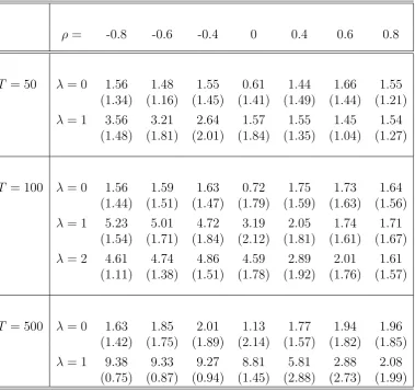
by Monte Carlo simulations. Table 1 summarizes the simulation results in terms of the

mean and standard deviation of the selected orders. Means and standard deviations

are computed based on 100 repetitions for each combination. Standard deviations are

provided in parentheses. The rows for λ = 0 correspond to models with no shift. By

inspecting the table, one concludes that a change in mean causes over estimation of

orders. The over estimation is particularly significant for negative ρ′_{s. For positive}

and large ρ′_{s, order selection is virtually unaffected by a shift. For example, for}

ρ = ₋.8, the average value of selected orders is 1.56 with no shift (λ = 0) and 3.56 with a shift (λ = 1); whereas for ρ = .8, the corresponding values are 1.55 and 1.54

respectively. The bias in order selection becomes larger as the number of observations

(T) increases. Consider the column for ρ = ₋.8, for instance, when the number of observations varies from 50 to 100 then to 500, the average selected orders are 3.56,

5.23, and 9.38 respectively (λ = 1). To see how the selected orders are distributed,

We plot histograms of the selected orders for two cases. Figure 3 plots the selected

orders when no shift exists (λ = 0). Figure 4 plots the counterpart when a shift does

exist (λ= 1).

6.3.

Order estimation based on generalized residuals

In the previous subsection, the shift is ignored and the order determination is based on

a misspecified model which leads to over estimation. Thus if a high order is identified in

practice, one should consider a possible parameter change. Tests should be performed

to test the parameter constancy. Many tests have been proposed in the literature

for testing parameter stability for time series models, for example, Andrews (1990),

Bai, Lumsdaine, and Stock (1991), Hansen (1990), MacNeill and Duong (1982), and

Ploberger, Kramer, and Alt (1989).

Table 1: Mean and Standard Deviation of Selected AR Orders

ρ= -0.8 -0.6 -0.4 0 0.4 0.6 0.8

T = 50 λ= 0 1.56 1.48 1.55 0.61 1.44 1.66 1.55

(1.34) (1.16) (1.45) (1.41) (1.49) (1.44) (1.21)

λ= 1 3.56 3.21 2.64 1.57 1.55 1.45 1.54

(1.48) (1.81) (2.01) (1.84) (1.35) (1.04) (1.27)

T = 100 λ= 0 1.56 1.59 1.63 0.72 1.75 1.73 1.64 (1.44) (1.51) (1.47) (1.79) (1.59) (1.63) (1.56)

λ= 1 5.23 5.01 4.72 3.19 2.05 1.74 1.71

(1.54) (1.71) (1.84) (2.12) (1.81) (1.61) (1.67)

λ= 2 4.61 4.74 4.86 4.59 2.89 2.01 1.61

(1.11) (1.38) (1.51) (1.78) (1.92) (1.76) (1.57)

T = 500 λ= 0 1.63 1.85 2.01 1.13 1.77 1.94 1.96 (1.42) (1.75) (1.89) (2.14) (1.57) (1.82) (1.85)

λ= 1 9.38 9.33 9.27 8.81 5.81 2.88 2.08

(0.75) (0.87) (0.94) (1.45) (2.88) (2.73) (1.99)

once a change point is estimated. Recall that the generalized residuals are defined as

ˆ

Xt=Yt−µ1ˆ −(ˆµ2−µ1ˆ )I(t >ˆk).

Because µ1, µ2, and τ can be consistently estimated we expect that order

determina-tion using the generalized residuals will remove, to some extent, the bias caused by

a shift. Figure 5 displays the selected orders based on the generalized residuals ˆXt.

Comparing with Figure 3, which is based on Xt, we find that the results are almost

Figure 1: Histogram of Estimated Change Points. Data is Generated According to:

Yt=µ+λI(t ≥k0) +Xt, with Xt=ρXt−1+εt+θεt−1, λ= 2, θ =.5, T = 100, and

Figure 2: Histogram of Estimated Change Points. Data is Generated According to:

Yt =µ+λI(t ≥ k0) +Xt, with Xt = ρXt−1+εt+θεt−1, λ= 2, θ = −.5, T = 100,

Figure 5: Selected Orders Via AIC Criterion Using Generalized Residuals ˆXt. Data is Generated According to: Yt =µ+λI(t ≥k0) +Xt, with Xt =ρXt−1+εt, λ= 1,

A

Appendix

Proof of (6). Write a∗

j = P

k≥j+1ak and Xt∗ = P∞

j=0a∗jεt−j. Under assumptions

(A or A′_{) and (B), X}∗

t is second-order stationary. Let σ12 =E(Xt∗)2 = σ2 P∞

j=0(a∗j)2. Then we have

Xt=a(1)εt−Xt∗+Xt∗−1, (A.1)

thus

ck k X i=1

Xi =a(1)ck k X i=1

εi+ckX0∗−ckXk∗,

where a(1) =P∞

j=0aj. Sinceck ≤cm for k≥m by assumption, we have

P r max

m≤k≤nck| k X i=1

Xi|> α !

≤P r max

m≤k≤nck|a(1) k X i=1

εi|> α/3 !

+ P r(cm|X0∗|> α/3) + P r

max m≤k≤nck|X

∗

k|> α/3

≤ 9σ

2_a(1)2 α2



mc2_m+ n X i=m+1

c2_i



 by H´ajek and R´enyi inequality

+ 9σ

2 1

α2 c

2

m+ n X i=m

c2_i

!

by Chebyshev inequality.

Hence if we chooseA= 9 max_{a(1)2_,P∞

j=0(a∗j)2}, then inequality (6) follows. Equation (A.1) is called the Beveridge-Nelson decomposition in the econometrics literature.

Phillips and Solo (1991) provide many interesting applications of this decomposition.

Proof of Proposition 1. Write ˆµ1(k) = 1_kPk_t=1Yt, then ˆµ1 = ˆµ1(ˆk). If k0 is known,

the LS estimation for µ1 is ˆµ1(k0). To prove (34), consider

T1/2µ1ˆ (ˆk)₋µ1ˆ (k0)=T1/2

  1 ˆ k ˆ k X t=1

Yt− 1 k0 k0 X t=1 Yt  

=I(ˆk _≤k0) 

T1/2

k0₋kˆ k0kˆ

k0 X t=1

Xt+T1/2 1 ˆ

k

k0 X

t=ˆk

Xt 



+I(ˆk > k0) 

T1/2

k0₋ˆk k0ˆk

k0 X t=1

Xt−T1/2 1 ˆ k ˆ k X t=k0

Xt+λT ˆ

k₋k0

ˆ

k





Now use k0 = T τ, ˆk = k0 +Op(λ−_T2), and T λ2

T → ∞, we find that the above is (T1/2_λ

the same limiting distribution. The latter has a limiting distribution given by the

right hand side of (34). The proof of (35) is similar.

Acknowledgments. This paper is based on Chapter 4 of my dissertation at the

University of California at Berkeley. I am grateful to my advisor, Professor Thomas

Rothenberg, for his encouragement and guidance throughout my study at Berkeley. I

am indebted to Professors Deborah Nolan and James Stock for their advice. I thank

professor Peter Bickel for invaluable discussions. Financial support from the Alfred P.

Sloan Foundation Dissertation Fellowship is gratefully acknowledged.

References

[1] Akaike, H. (1974) A new look at the statistical model identification. I.E.E.E.

Trans. Auto. Contr. Ac-19, 716-723.

[2] Andrews, D. W. K. (1990) Tests for parameter instability and structural change

with unknown change point. Manuscript, Cowles Foundation, Yale University.

[3] Bai, J., Lumsdaine, R. L., and Stock, J. H. (1991) Testing for and dating breaks

in integrated and cointegrated time series. Manuscript, Kennedy School of

Gov-ernment, Harvard University.

[4] Bhattacharya, P. K. (1987) Maximum likehood estimation of a change-point in

the distribution of independent random variables: General Multiparameter case.

J. of Multivariate Analysis 23, 183-208.

[5] Birnbaum, Z. W. and Marshall, A. W. (1961) Some multivariate Chebyshev

in-equalities with extensions to continuous parameter processes. Ann. Math. Stat.

32, 687-703.

[6] Chung, K. L. (1968) A Course in Probability Theory. Harcourt, Brace & World

[7] H´ajek, J. and R´enyi, A. (1955) Generalization of an inequality of Kolmogorov.

Acta. Math. Acad. Sci. Hungar. 6, 281-283.

[8] Hall, P. and Heyde C. C. (1980) Martingale Limit Theory and its Applications.

New York: Academic Press.

[9] Hansen, B.E. (1990). Testing for structural change of unknown form in models

with non-stationary regressors. manuscript, University of Rochester.

[10] Hawkins, D. L. (1986) A simple least square method for estimating a change in

mean. Commun. Statist.-Simul. 15, 655-679.

[11] Hawkins, D. M. (1977) Testing a sequence of observations for a shift in location.

J. of American Statistical Asso. 72, 180-186.

[12] Hinkley, D. (1970) Inference about the change point in a sequence of random

variables. Biometrika 57, 1-17.

[13] James, B., James, K., and Siegmund, D. (1987) Tests for a change point.

Biometrika 74, 71-83.

[14] Kim, J. and Pollard, D. (1990) Cube root asymptotics. Annals of Statistics 18,

191-219.

[15] MacNeill, I. B. and Duong, Q. P. (1982) Effect on AIC-type criteria of change of

parameters at unknown time. In Time Series Analysis: Theory and Practice 1,

edited by O.D. Anderson. North-Holland Publishing Company.

[16] Picard, D. (1985) Testing and estimating change-points in time series. J. Applied

Prob. 14, 411-415.

[17] Phillips, P. C. B. and Solo, V. (1989) Asymptotics for linear processes. Cowles

[18] Ploberger, W. K., Kramer W., and Alt R. (1989) A modification of the CUSUM

test in the linear regression model with lagged dependent variables. In W. Kramer

(ed.) Econometrics of Structural Change. Physica-Verlag, Heidelberg.

[19] Sen, A. and Srivastava, M. S. (1975a) On tests for detecting change in mean.

Ann. stat. 3, 96-103.

[20] (1975b) Some one-sided tests for change in level. Technometrics 17,

61-64.

[21] Srivastava, M. S. and Worsley, K.J. (1986) Likelihood ratio tests for a change in

the multivariate normal mean. J. Amer. Stat. Asso. 81, 199-204.

[22] Worsley, K. J. (1979) On the likehood ratio test for a shift in locations of normal

populations. J. of the American Statistical Association72, 180-186.

[23] (1986) Confidence regions and tests for a change-point in a sequence of

exponential family random variables. Biometrika 73, 91-104.

[24] Yao, Y. C. (1987) Approximating the distribution of the ML estimate of the

change-point in a sequence of independent r.v.’s. Annals of Statistics 3,