Deploying State Space Control to Regulate an Inverted Rotary Pendulum with Non Zero Input

© 2016, IRJET | Impact Factor value: 4.45 | ISO 9001:2008 Certified Journal | Page 9

DEPLOYING STATE SPACE CONTROL TO REGULATE AN INVERTED

ROTARY PENDULUM WITH NON-ZERO INPUT

Bui, Hoang Dung

Department of Mechanical Engineering and Material Science, Faculty of International Training,

Thai Nguyen University of Technology, 666, 3-2 Street, 251812 Thai Nguyen City, Vietnam

---***---Abstract -

State space control has a wide application for

multiple inputs and multiple outputs systems. In several researches, it is used to control Inverted Rotary Pendulum (IRP) whose reference inputs are zero. In this paper, this control algorithm is deployed to regulate an IRP working when the arm is at non-zero position. The controlling challenge is the IRP state vector has to be extended to deal with the arising error. As consequently, the IPR’s parameter matrices are also expanded to handle with the new vector. Base on that, a state space control law is built to implement the regulation by LQR method. The calculated control law is tested by simulation and experiments. The results present the availability of the LQR approach in controlling the IRP with nonzero input.

Key Words: Non-zero Input, State Space Control, LQR, Inverted Rotary Pendulum

1.INTRODUCTION

Inverted Rotary Pendulum (IRP) is a nonlinear under-actuated mechanical system which is well-suited to verify and practice the ideas of control theory [1][2]. There were several control methods applied on IRP models and their responses to hold the pendulum at upright position were good. [1]-[5].

In some researches, real IRP models were built and controlled by some control methods such as State Space Control, PID, Fuzzy Control [3]-[5]. Those control algorithms regulated the IRP and stabilized it when the pendulum is at the upright position. However, all the researches have only focused on controlling the IRP as its arm stays at the zero position. It means the arm can work only in one position in the whole operating range (0o _{÷ 360}o_).

This paper is to find a way to regulate the IRP to work with non-zero input for the arm position. In order to do that, State Space Control method is used to determine a control law. To handle with the error causing by the nonzero position of the arm, one more state is added to the IRP state vector, increasing the considered states into five. This will make the controller more complicated.

In the following sections, we will set up the dynamic equation systems of the IRP, establish an appropriate control

law, build a model and simulate it, and finally make experiments by applied the control law in a real IRP.

2. IRP’s DYNAMIC EQUATION SYSTEM

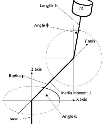
IRP consists of two rotary axes whose positions are the two system’s outputs. Its structure is shown in the Fig - 1 with an arm with length ρ and a pendulum bar l rotating around the Z-axis and Y-axis. The rotation of the arm and bar are called angles α and , respectively. In steady state, the mass m stays at the upright position ( = 0) and the arm’s position α

[image:1.595.341.523.394.606.2]

stands at a desired position.

Fig - 1: An IRP structure

The pendulum is driven by a DC motor via a gearbox and a belt transmission. As angles α and φ change, the differences between the values and the desired inputs are used as the input for the controller. With the parameters above, the IRP dynamic equations have built by author’s master thesis [6], and the results are presented here:





    

 

 

 

 

 



0 sin )

cos sin ( ) cos (

) cos sin 2 (

) sin ( ) cos ( sin

2 2

2

2

2 2

2 2

 

  

  

   

        

mgl ml

l m ml

M ml

l m l

m ml

m J

in

 

 



 

 

 



© 2016, IRJET | Impact Factor value: 4.45 | ISO 9001:2008 Certified Journal | Page 10

Min is the torque driven from DC motor.

The IRP only works around the upright position with small deviation and α varies slowly around desired position. Therefore an approximated model is built by linearization around the working point. Before doing that, a state vector is established by introducing some new variables (α1, 1, α2,

2):

        _{    }  2 2 1

1 ; ; ;

       _{ }  _{  }  _

 1 2; 1 2; 2 ; 2

Introduce state vector x:

T

x[₁ ₁ ₂ ₂] (2)

Linearizing the equation system (1) around the working point ( 0; α 0), sin 0; sinα  0, cos 1; cosα 1, results in:





in

M Jl J Jl g m J J g m _                                                                        1 0 0 0 0 0 0 0 2 0 1 0 0 0 0 1 0 0 2 2 1 1 2 2 2 1 1     (3)

[image:2.595.310.519.225.303.2]

Combination with DC motor and gearbox: The IRP is driven by a DC motor with gearbox and belt transmission which are shown in Fig - 2:

Fig - 2: DC motor circuit with gearbox - belt transmission From the DC motor electrical circuit and the transmission via gear box and the belt, the relationship between the input voltage, arm angle α1 and Min is:

1 2

1







_ m m m m in R K K V R K

M   (4)

where  = gmb, K1 = KgKbKt; K K_g2K_b2K_t

2  .

(Rm: resistance of the motor, Vm,: supplied voltage, Min,: output

torque of the belt transmission, m, b, g: efficiencies of DC

motor, belt transmission, gearbox, Km, Kt: motor & torque

constant, Kb, Kg transmission ratios of the belt and gearbox) Substitute Equation (4) into Equation (3):

m

V

P

P

P

P

P

P













































































































6 5 2 2 1 1 4 2 3 1 2 2 1 1

0

0

0

0

0

0

1

0

0

0

0

1

0

0

























(5) where J g m

P₁2  ;





Jl g m J P 2 2  

 ; 2 ;

3 m m JR K K

P 

; 2 4 m m JlR K K

P   1;

5 m

JR K P 

m JlR K P 1 6  

As the dynamic equations get done, the features of the IRP can be verified.

3. CONTROL LAW

Before finding out an appropriate control law, the IRP is inspected for controllability and observability.

Introducing matrices

A

,

B

, and

C

:

; 0 0 0 0 1 0 0 0 0 1 0 0 4 2 3

1 _

             P P P P A              6 5 0 0 P P

B ; _

     0 0 1 0 0 0 0 1 C ;

3.1 Controllability

It is a property, which enables one to steer the dynamic system to a desired trajectory [8]

The IRP system is controllable if and only if the matrix



B

A

B

A

B

A

B



Q

c

3 2



is non-singular [8].

The controllability of IRP is checked at section 4 when all parameters are substituted in the formula.

3.2 Observability

Itis a property, with which the system state trajectory can be deduced from the input and output trajectories [8]. The IRP is observable if and only if the matrix

Where





T

o C CA CA CA

Q  2 3

is non-singular [8].

Multiplying two matrices

C

and

A

with the form above,

lead to:                                2 1 4 3 2 3 4 3 4 1 3 1 2 1 0 0 1 0 0 0 0 1 0 0 0 0 1 0 0 0 0 0 0 0 0 1 P P P P P P P P P P P P P Q o Rank( o

Q ) = 4, so o

Q is non-singular and the IRP system is

© 2016, IRJET | Impact Factor value: 4.45 | ISO 9001:2008 Certified Journal | Page 11

3.3

Establishing an appropriate control law

The control parameters K is calculated by LQR approach with Matlab function lqr(). The function’s inputs are four matrices:

A

, B, Q and R, the last two matrices are used to

balance the effort and responses of the system.

To control the IRP at a non-zero position of the arm, there is a new state added to the State Vector (2).

Introduce a new variable e:

e = α1 – r (6) where r is a non-zero desired position of the arm.

Differentiating Equation (6):

2 1







 



e (7)

Introduce another new variable xI with: e

x_I  (8)

A new state vector xN is created by combining the State Vector (2) and the new one xI:





T

I

N x

x 1 1 2 2

Because of changing the state vector, the IRP model can now be expressed as

r N N N

N A x B u

x  

And their new parameters:

     

 

     

 

  

0 0 0 0 1

0 0 4 2 0

0 0 3 1 0

0 1 0 0 0

0 0 1 0 0

P P

P P A

N

;

     

 

     

 



0 6 5 0 0

P P B_N

with five states and one input, the matrices _Q andR have

dimension 5x5 and 1x1. The control law is adjusted by the educated trail-and-error-repetition technique until the performance of the controlled system is stable within 3 seconds. The adjustment gets done by changing the matrices

Q

and

R

. After check and error, the most appropriate

values of two matrices

Q

and

R

are:

]) 1 , 5 . 0 , 2 . 0 , 2 , 5 . 0 ([

diag

Q

;

R = 0.5;

Applying lqr() function with the parameters above to find the control law.

K = lqr(AN, BN, Q, R)

4. MODELING AND SIMULATION

Based on the dynamic equation and control law, the model is built on MatLab-Simulink.

4.1

Modeling

To ease the understanding, components of the IRP equations are grouped into a subsystem called PLANT. The others two parts are the integral one and feedback one. The structure is shown in the Fig - 3.

The states are multiplied with their own control parameters

[image:3.595.41.241.461.546.2]

K1, K3, K2, K4 and K5. The first four ones belong to Feedback part whose inputs are four states (positions and angular velocity of pendulum and arm) and its output is a part of feedback signal.

Fig – 3: Closed Loop Model

4.2

Simulation

Based on a real IRP, the parameters for the Simulink - model are:

Kt= 0.02 Nm/A, l = 0.3m, m = 0.03Kg, ηb = 0.98, J = 0.002

Kgm2_{, g = 0.98, ηm = 0.51, g = 9.8 m/s}2_{, Rm =}

3Ohm, Kg = 18, Km = 0.02 Vs/rad, Kb = 4.

Substituting the system parameters to calculate the coefficients of the matrices

A

and

B

:

2 1 36.4 1_s

P  ; P2 40.61_s2;

s rad P

 161.2 1 3

rad s P

 69.9 1

4 ; 5 2

1 9 . 111

Vs

P  ; P6 48.5 1_Vs2

The next step is to check the IRP’s controllability. Using the

det() function from MatLab:

 

2.36 8 0

detQ  e 

c

;

Hence, rank( c

Q ) = 4 and the IRP is controllable.

© 2016, IRJET | Impact Factor value: 4.45 | ISO 9001:2008 Certified Journal | Page 12

Using lqr() function to get the control law:

K = lqr(AN, BN, Q, R)

K = [-2.92 50.5 -4,1 10,1 -1,41]T

With these parameters, the IRP’s stability needs to be verified. The system is stable if and only if all the poles and zeros are negative [8]. The poles and zeros are determined by function eig():



A B K



eig

ZP

N

N  



ZP=[-182.7 -0.7+0.6i -0.7-0.6i -4.9+0.6i -4.9-0.6i]T The found result meet the mentioned condition, therefore the controlled IRP is stable.

To simulate the model, there are several prerequisites. Firstly, the controlled IRP only works in a small range (-0.16 ÷ 0.16) rad around the upright position and the mass M’s velocity is small (≤ 0.4m/s). The initial conditions for the model are: The desired inputs: α = 0.4 rad;  = 0 rad, the initial positions of angles α0= 0.15 rad; 0 = 0.1 rad and two initial angular velocities 00m/s, 0 0.1m/s.

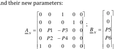
The IRP model’s responses are shown in Fig-4 and 5. The horizontal and vertical axes represent the simulation time (second) and the angle values (rad), respectively. Fig - 4 presents the behavior of the arm. From initial position α0=

[image:4.595.309.560.73.251.2]

0.15 rad, it moves rapidly to the negative position to hold the mass M at the upright position. When the mass M is stable, the pendulum’s arm reaches its desired position α0= 0.4 rad after 2.8 seconds.

Fig – 4: Angle α response

[image:4.595.314.547.466.635.2]

Fig-5 shows the behaviors of the mass M. From initial position 0 = 0.1 rad, it moved to the upright position and stayed there after 0.8 seconds.

Fig – 5: Angle  response

5. EXPERIMENT AND RESULTS

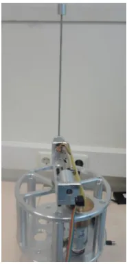
After the simulation, the control law is applied to a real IRP (Fig. 7) whose parameters are mentioned on previous section. The machine is controlled by four microcontrollers (uC) AT90CAN128. The arm and pendulum angles are measured by two optical encoders which have 2000 values/revolution. The communication among these microcontrollers is done by TTCAN protocol.

The positions of the two angles during the IRP operation are transmitted to a computer via uC’s USART port and a Hterm

device. These data are plotted graphically by software

Gnuplot.

Fig – 6: A real model of IRP

At non-operation state, the pendulum is at right-down position and its angle is set to “0”. At stable working condition, the pendulum should stay at upright range (171o _÷

189o_{) or (-189}o _{÷ 171}o_{) and the values of the pendulum’s}

encoder should be in (910÷1090) or (-1090÷ -910). To move the pendulum into the upright range, the DC motor supplies kinetic energy to the pendulum and make it oscillating with increasing magnitude. Since the pendulum reaches the Upright range, the IRP controller switches to the Upright

[image:4.595.39.275.511.685.2]

© 2016, IRJET | Impact Factor value: 4.45 | ISO 9001:2008 Certified Journal | Page 13

established in the previous section) to regulate the

pendulum stay in that range.

[image:5.595.307.563.67.227.2]

The Fig-7 and 8 present graphically positions of the pendulum and the arm from the experiment. The data were collected from the encoders and processed by a computer. The time is counted by uC’s counters and presented by the horizontal axes. Each counter value is equal to 2 msec.

Fig – 7: The Pendulum is in Upright range after oscillating with increasing amplitude

The Fig - 7 shows the pendulum position from oscillating with increasing amplitude to reach the Upright range then stays in that range. The vertical axis presents the position of the pendulum (from the pendulum’s encoder with the value range from -1999 to +1999). The time to get the data starts at the value 6000. Starting from the zero position, the DC motor had driven the pendulum to swing up. After several oscillations, the pendulum had enough energy to go to the Upright range. In that range, the IRP switches to Upright phase and uCs use the calculated control law to regulate the pendulum stays at that range steady. The pendulum position still stays stable in this range even though the arm position varies.

The Fig - 8 presents the arm position with nonzero reference input. When the pendulum was at the upright position, the new position of the arm was set to -210_{, which was equal the}

encoder’s value -117. As the new reference input was applied, the arm moved slowly to the new position. The movement was not smooth but oscillating then reached the desired position at the counter value 5000. After that, the arm still oscillated but around the new position steady with decreasing amplitude. From the time of 25000, the amplitude of arm oscillation is stable about 2.7o _{(the encoder}

[image:5.595.39.286.190.323.2]

values are from 111 to 126).

Fig - 8: The Arm position in Upright phase with nonzero reference input

There are two reasons for that phenomenon. The first one is the gearbox’s backlash (around 0.50_{), which makes the arm}

loss amount of motion as the DC motor reverse the movement’s direction. That caused the arm slipped out the predefined amplitude and oscillated longer to reach the upright point. The second reason is the parallel misalignment between the shaft of the gearbox and the arm rotation axis, which makes the inconstant transmitted torque between the gearbox and arm rotated axis. It also creates the vibration of the arm axis.

The Fig - 9 showed the IRP in the Upright State when the arm position was set to -210

Fig – 9: The IRP at upright position

6. CONCLUSIONS

[image:5.595.387.480.416.608.2]

© 2016, IRJET | Impact Factor value: 4.45 | ISO 9001:2008 Certified Journal | Page 14

requirements. The result proves the robustness of the

control method in the SIMO system.

REFERENCES

[1] Jadlovska S., Jan Sarnovsky J., A Complex Overview of Modeling and Control of the Rotary Single Inverted Pendulum System - POWER ENGINEERING AND ELECTRICAL ENGINEERING, VOLUME 11-2, 2013, pp. 73-85

[2] Sirisha V., Junghare A. S. – A comparative study of controllers for stabilizing a Rotary Inverted Pendulum

-International Journal of Chaos, Control, Modeling and Simulation (IJCCMS), Vol.3, No.1/2, DOI : 10.5121/ijccms.2014.3201 , June 2014

[3] Jose A., Augustine C., Malola S. M., Chacko K., -

Performance Study of PID Controller and LQR Technique for Inverted Pendulum - World Journal of Engineering and Technology, 2015, 3, pp. 76-81

[4] Babu J., Varghese E., Stabilization of Rotary Arm Inverted Pendulum using State Feedback Techniques - International Journal of Engineering Research & Technology (IJERT) ISSN: 2278-0181, Vol. 4 Issue 07, 2015, pp.563-567 [5] Hassan M., Kadri M., Amin I., Proficiency of Fuzzy Logic

Controller for Stabilization of Rotary Inverted Pendulum based on LQR Mapping – Fuzzy Logic and Applications: 10th _{International Workshop, WILF 2013, Italy, pp.}

201-211

[6] Bui, D. H. - Development and Realization of a distributed control algorithm for an inverted rotary pendulum using FreeRTOS with TTCAN communication, Embedded system Institute, University of Siegen, 2014

[7] Franklin G. F. J., Powel D., Emami-Naeini A.– Feedback control of Dynamic System 5th Pearson Education, Inc, 2006, New Jersey, - ISBN 0-13-149930-0, pp 438-563 [8] Polderman J. W., Willens J. C., Introduction to the

Mathematical Systems Theory: A Behavioral Approach,

Spinger Verlag 1998, ISBN 978-1-4757-2953-5, New