An algorithm for solving cost time trade-off pair in quadratic fractional
transportation problem with impurity restriction
Nidhi Verma Arya
1, Preetvanti Singh
21,2 Department of Physics and Computer Science,
Faculty of science Dayalbagh Educational Institute Dayalbagh, Agra, India
---***---Abstract
- In many real life transportation situations like industries of coal, iron and cement. The commodity does vary in some characteristics according to it source. The final commodity mixture reaching the various destinations may then be required to meet known specifications. It has also been observed that time of transportation is as important as cost of transportation. Generally the optimal solution for time minimizing transportation problem may not be unique and a number of transportation solutions will consume the same optimal time of transportation. So out of these solutions it is quite difficult to choose best solution with respect to second criteria i.e. the transportation cost. This gives rise to the problem of obtaining cost and time trade-off pair. Cost-time trade-off problems have been studied for a number of linear transportation problems. The focus of this paper is to develop an algorithm for generating trade-off pairs between cost and time for quadratic fractional transportation problem with impurity restriction. The algorithm will generate all the solutions which are pareto optimal with respect to transportation cost and the transportation time.Key Words: quadratic transportation problem, trade-off, impurity constraint, algorithm, optimality conditions.
1. INTRODUCTION
Optimizing transportation problem has a significant role in real-life situations. Different variants of this problem is available in literature. Quadratic transportation problem is a special type of Quadratic programming problem which can be stated as a distribution problem where each of the m suppliers can ship units to any of the n customers at cost ) and where is a quadratic function of the amount shipped from source i to destination j. The objective of the Quadratic transportation problem is to minimize the total transportation cost while meeting demand at the destinations. Transportation problem with fractional objectives occur in many real-life situations where the objective function includes optimization of ratio of total actual transportation costs to total standard transportation cost, total return to total investment, ratio of risk assets to capital etc. A Transportation problem with fractional objective function was investigated by Charles, Yadavalli, Rao, & Reddy (2011) as a stochastic programming model, while considering ratio of two non-linear functions and probabilistic constraints. Sivri, Emiroglu, Güzel & Tasci (2011) dealt with the transportation problem of minimizing the ratio of two linear functions subject to constraints of the
convention transportation problem. Gupta & Arora (2013) studied linear plus linear fractional capacitated transportation problem with restricted flow. Khurana & Arora (2013) formulated a transportation problem with an objective function as the sum of a linear and a linear fractional function with restricted enhanced flow. The linear function represents the total transportation cost incurred in shipping goods from various sources to the destinations and the fractional function presents the ratio of sales tax to the total public expenditure. Das, Mandal & Edalatpanah (2017) proposed a new approach for solving fully fuzzy linear fractional programming problems using the multi-objective linear programming. Time transportation problem is an important problem from the practical point of view and its study is of great interest. Chakraborty & Chakraborty (2010) proposed a method for the minimization of transportation cost as well as time of transportation. Singh (2012) developed a procedure for providing the optimal solution to quadratic time transportation problem. An algorithm was developed by Uddin (2012) to determine the minimum transportation time. Quddoos, Javaid, Ali, & Khalid (2013) considered a bi-objective transportation problem, where the total transportation cost and delivery time was minimized. These problems consider optimization of only one objective cost or time. However in real-life problems the trade-off between cost and time also plays an important role. Li, Shi & Jhao (2001) proposed a method for time-cost trade-off in a transportation problem with multi-constraint levels. Basu, Pal & Kundu (2007) developed an algorithm for the time-cost trade-off in fixed charge bi-criterion transportation problem. An algorithm for finding time-cost trade-off pairs in generalised bi-criterion capacitated transportation problem was presented by Das, Acharya & Basu (2015). Sharma & Arora (2017) discussed modification on a cost pipeline trade-off in a transportation problem. In the present a new type of optimization problem is considered by integrating quadratic transportation problem, fractional transportation problem, time transportation problem and impurity restriction. In some practical applications, the product varies in some features according to its source. The final product mix, received at destinations, may then be required to meet known specifications. For example, crude ore contains different amounts of phosphorus impurity, according to its source and the actual time to process the ore depends on both its source and destination. This type of transportation problem is studied by Haley and Smith (1966), and Saxena, Singh & Saxena (2013).
1.1 The quadratic fractional transportation with bottleneck time and impurity restriction (QFTTPI)
This section presents the formulation of the quadratic fractional time transportation problem. The objective function is quadratic and fractional with linear constraints. The mathematical formulation of the problem is as follows: Let there be M sources and N destinations.
be the quantity of the commodity available at the ith source
and be the quantity of commodity required
at the jth destination. be the amount of the commodity transported from the ith source to the jth destination. Let C= ], and D= ] be the two (M×N) cost matrices and E= [ be a (M×N) time matrix. is the unit actual shipping cost, is the unit standard shipping cost. be the shipping time of the commodity from the ith source to the jth destination, and is independent of the commodity transported for ≥ 0. denotes the units of P impurities (k=1,…, P) that one unit of the commodity contains when it is sent from ith source tojth destination. Destination j cannot receive more than units of impurity. α, β are scalars and constants. The problem is to find a trade-off between two the objectives, the total shipping cost ratio Z and earliest shipment completion time T, over the entire range of the feasible solutions, where Z and T are stated as:
subject to constraints
In this problem the quadratic transportation problem with objective function as (1) and constraints (3) to (6) will be denoted by Q.
Here
There are a total of MN+NP variables including slacks and NP+M+N equations. By imposing conditions on the and the , one of the equations (3) and (4) is dependent and so a basic feasible solution will consist of NP+M+N-1 basic variables.
The impurity restriction can be written as: Where
are the slack variables to impurity restrictions.
2. Methodology and the algorithm
In this section, an algorithm is developed for finding all optimal schedules with earliest shipment completion times less than successively till no other feasible schedules are to be found on the permissible routes, where
The set of positive variables in the kth optimal solution and is one of the K alternative optimal solutions with optimal value to the problem Q. Any transportation schedulewith minimum cost ratio cannot have completion time less than and any transportation schedule which is completed earlier than time will have cost ratio more than .
Definition 1- T is said to be a feasible time for the problem Q, if there exists a feasible solution X for the problem Q, with . Otherwise, T is said to be an infeasible time for the problem Q.
Definition 2- A solution pair is said to be an efficient solution pair (or pareto-optimal solution pair) if there exists no other solution pair (Z,T) such that
(i) and
or (ii) and
Denote initially Q, , and by and respectively.
3. The algorithm to solve QFTTPI is given below
The stepwise description of thealgorithm is now as follows:
Step 1: Determine optimal solution to the problem
Q
0using the following sub-steps:Step 1a: Find the initial basic feasible solution to the problem
0
Q
by the method of Singh and Saxena [2].Step 1b: Determine the dual variables and 1 ij
w
, 2ij
w
such thatfor all basic cells.
Step1c: Evaluate
For all non-basic cells. Where
And = and =
Step 1d: If for non-basic variables, all ,
M k j ,
0
current basic feasible solution is optimal which implies going to Step 1 (g). Otherwise go to Step 1 (e) to improve the solution.Step 1e: Choose the most negative of the which
ij;
M k j , which may be designed by0 0 i j
or0,0 M k j
and determinethe variable
0 0 i j
x
or0,0 M k j
x
which is to enter. The variable0 0 i j
x
or0,0 M k j
x
then becomes a basic variable of the new basic feasible solution.Step 1f: Change the current solution to the new basic feasible solution using equations [11]:
Furthermore, the values of the variables in the updated basic
feasible solution are given by ;
. Choose a suitable value of from
M ys
s y M
rs rs
n
n
n
x
n
x
s y M rs
, ,
0
;
min
0 ,
(23)and go to step 1b.
Step 1g: The optimal solution gives the optimal
transportation schedule
Step 2:Obtain * 0
Z
and * 0T
. Note that in case problemQ
0 has alternative optima, *0
T
will be computed from equation(10), otherwise
* *
0 ( , )
max
ij/
ij0
i jT
t
x
(24)
Now use the same notation, that is, *
X
for those alternative optima, (in case there is one) for which *0
T
has been computed by equation (10).Step 3: Modify the cost matrices as follows to get the problem
Q
1:(25)
(26)
For all i and j.
(18)
(19)
Step 4: Replace in by and in by and use the optimal solution of
Q
0 to optimizeQ
1. Step 5: If Q has a feasible solution for the permissible routes, then a new value and a new value is obtained such that and . Continue iterations yielding ( , ), ( , ),…,till no other feasible solutions are to be found on the permissible routes.4. Case study
The above Algorithm is illustrated with the help of a raw material (cement) shipping problem. A cement manufacturing unit has different types of cement processing sections in each of four work centres (j). The WorkCentre j
are receiving a fixed quantity of raw material (i), which has three different grades. Due to technical reasons, the processing time of raw material depends on its grade and the workcentres to which it is sent. The problem is to determine a feasible transportation schedule which minimizes the ratio of total actual shipping cost and total standard shipping cost of raw material , and also minimizes the maximum of shipping time of raw material, while satisfying the extra requirement that the amount of sulphur tri-oxide impurity present in crude raw material is less than a critical level.
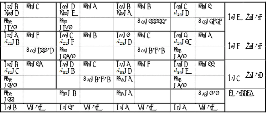
In Table 1, and is written on the top left corner of the cell.
t
ij is shown in upper right corner of the cell. and the impurities are given in the last two columns respectively, [image:4.595.298.582.137.386.2]and maximum sulphur tri-oxide contents are shown in the last row.
Table 1: Data for the Problem Q0
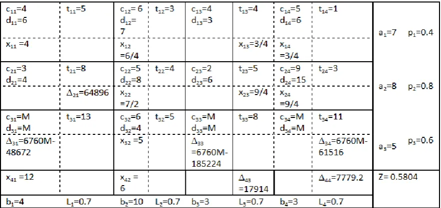
The optimal solution for problem is shown in Table 2.
Table 2: Optimal Solution to c11=
4 d11=
6
t11=
5 c6 12= d12=
7
t12=
3 c4 13= d13=
3
t13=
4 c14=5 = 6
t14= 1 a1 =7 p 1 = 0 . 8 c21=
3 = 4
t21= 8 c5 22=
= 8
t22= 4 c2 23=
= 6
t23=
5 c24=9 = 15
t24= 3 a2 =8 p 2 = 0 . 8 c31=
4 = 5
t31= 13 c6 32=
= 4
t32=
5 c3 33= = 6
t33=
8 c34=6 = 7
t34= 11 a3 =5 p 3 = 0 . 6 b1=
4 0.7 L1= b10 2= L0.7 2= 3 b3= L0.7 3= b4=3 L0.7 4=
c11=4
d11=6
t11=5 c12= 6
d12= 7
t12=3 c13=4
d13=3
t13=4 c14=5
=6 t14=1
a1=7 p1=0.8 x11
=7/2 x=7/2 12 13=112110 14=9898
c21=3
=4 t21=8 c22=5 =8 t22=4 c23=2 =6 t23=5 c24=9 =15 t24=3
a2=8 p2=0.8
21=61206 x22
=13/2 23=40804 x=3/2 24
c31=4
=5 t31=13 c32=6 =4 t32=5 c33=3 =6 t33=8 c34=6 =7 t34=11
a3=5 p3=0.6 x31
=1/2 32=40804 x33 =3 x=3/2 34
x41
=11 x42 = 4 x43 =3 34=202 Z= 0.4473
b1=4 L1=0.7 b2=10 L2=0.7 b3=3 L3=0.7 b4=3 L4=0.7
[image:4.595.85.512.497.679.2]Table 3: Optimal Solution to
Table 4: Optimal Solution to Q2
Table 5: Optimal Solution to Q3
c11=4 d11=6
t11=5 c12= 6 d12= 7
t12=3 c13=4 d13=3
t13=4 c14=5
=6 t14=1
a1=7 p1=0.8
x11 =4 x12 =3 13=108108 14=10296
c21=3
=4 t21=8 c22=5 =8 t22=4 c23=2 =6 t23=5 c24=9 =15 t24=3 a2=8 p2=0.8
21=58806 x22 =7 23=39600 x24 =1
c31=M
=M t31=13 c32=6 =4 t32=5 c33=3 =6 t33=8 c34=6 =7 t34=11
a3=5 p3=0.6
31
=9702M-19602 32=38808 x=3 33 x34 =2
x41 =12 x42 =
2 x=3 43 x44 =1 Z= 0.4474
b1=4 L1=0.7 b2=10 L2=0.7 b3=3 L3=0.7 b4=3 L4=0.7
c11=4
d11=6
t11=5 c12= 6
d12= 7
t12=3 c13=4
d13=3
t13=4 c14=5
=6 t14=1
a1=7 p1=0.8
x11 =4 x12
=9/4 13=158208 x=3/4 12
c21=3
=4 t21=8 c22=5 =8 t22=4 c23=2 =6 t23=5 c24=9 =15 t24=3
a2=8 p2=0.8
21=63654 x22
=23/4 23=84872 x=9/4 24
c31=M
=M t31=13 c32=6 =4 t32=5 c33=3 =6 t33=8 c34=M =M t34=11
a3=5 p3=0.6
31
=9682M-59946
x32 =2 x33
=3 83224 34
=9682M-x41 =12 x42 = 3 x43
=3 44=3811 Z= 0.4743
b1=4 L1=0.7 b2=10 L2=0.7 b3=3 L3=0.7 b4=3 L4=0.7
[image:5.595.78.520.513.722.2]Here ( , ) =(0.4473, 13) . Redefine the costmatrices as follows to get the problem :
The modified cost matrices for is given in Table 3 with the resulting optimal solution .
In this case the optimal values are ( = (0.4474, 11). Now redefine the cost matrices [ ] and [ ] as follows to get the problem :
[image:6.595.305.570.61.235.2]
for all i and j.
Table 4 has the new cost matrices for Q2 and also the optimal
solution .
The optimal values are ( = (0.4744, 8). Again redefine the cost matrices [ ] and [ ] as follows to get the problem
:
for all i and j.
The unique optimal solution to the problem is shown in Table 5.
In this case the optimal values are ( = (0.5804, 5). A furthermodification of cost matrices result in there being no feasible solution. Therefore, the algorithm terminates.The minimum total cost ratio shipping time combinations, as obtained by the algorithm are (0.4473,13), (0.4474, 11), (0.4744, 8) and (0.5804, 5) . This gives a picture of the trade-offs that have been madeand are represented in Figure 1. It can be seen that a successive reduction in the earliest completion time is there at the cost of an increasein the minimum total fuel cost ratio.
Figure 1: The cost-time trade-off
5. Conclusion
The main objective of this paper is to develop an algorithm to obtain the solution frontiers of the cost-time trade-offs in the quadratic fractional transportation problem with bottleneck time and impurity restriction. The algorithm is useful in cases not only where the time-objective is an equally crucial factor besides cost ratio, but also when analyzing the practicability of an existing transportation system. This procedure helps the decision maker by eliminating all the inefficient solutions. The developed methodology will prove to be useful in making the transportation problem formulation more realistic in applications areas.
6. References
[1] Haley K.B & Smith A.J (1966) Transportation Problems with Additional Restrictions, Journal of the Royal Statistical Society Series C (Applied Statistics),15(2), 116-127.
[2] Singh P & Saxena P. K (1998) Total shipping cost/completion-date trade-offs in transportation problems with Additional Restriction, Journal of Interdisciplinary Mathematics, 1 (2-3), 161-174.
[3] Li J, Shi Y, & Jhao J (2001) Time-cost trade-off in a transportation problem with multiconstraint levels, 5, 11-20.
[4] Basu M, Pal B.B & Kundu A (2007) An algorithm for the optimum time-cost trade-off in fixed-charge bi-criterion transportation problem bi-bi-criterion transportation problem, A Journal of Mathematical Programming and Operations Research, 30(1), 53-68.
[5] Charles V, Yadavalli V.S.S, Rao M.C.L, & Reddy P.R. (2011) Stochastic Fractional Programming Approach to a Mean and Variance Model of a Transportation Problem. Hindawi Publishing Corporation Mathematical Problems in Engineering, 1-12.
[image:6.595.70.249.121.200.2][6] Sivri M, Emiroglu I, Güzel C, & Tasci F (2011) A solution proposal to the transportation problem with the linear fractional objective function. In: Proceedings of Modelling, Simulation and Applied Optimization (ICMSAO), 2011 4th International Conference on, 1921 April 2011, Kuala Lumpur, 1–9. DOI: 10.1109/ICMSAO.2011.5775530.
[7] Uddin M. S. (2012) Transportation Time Minimization: An Algorithmic Approach. Journal of Physical Sciences, 16:59-64.
[8] Gupta K & Arora S.R (2013) Linear Plus Linear Fractional Capacitated Transportation Problem with Restricted Flow, American Journal of Operations
Research, 3(6), 581-588.
DOI: 10.4236/ajor.2013.36055
[9] Khurana A & Arora S.R (2013) The sum of a linear and a linear fractional transportation problem with restricted and enhanced flow, Journal of Interdisciplinary Mathematics, 9(2), 373-383.
[10] Quddoos A, Javaid S, Ali I & Khalid M. M (2013) A Lexicographic Goal Programming approach for a bi-objective transportation problem. International Journal of Scientific & Engineering Research, 4(7), 1084-1089
[11] Saxena A, Singh P & Saxena P.K (2013) Quadratic fractional transportation problem with additional impurity restrictions. Journal of Statistics and Management Systems, 10(3), 319-338, DOI: 10.1080/09720510.2007.10701257
[12] Das A, Acharya, D & Basu M (2015) An algorithm for finding time-cost trade-off pairs in generalised bi-criterion capacitated transportation problem, International Journal of Mathematics in Operational Research, 7(4)
[13] Singh P (2015) Multi-objective fractional cost transportation problem with bottleneck time impurities. Journal of Information and Optimization Sciences, 36(5), 421-449,
[14] Sharma S & Arora S (2016). Limitation and modification: On a cost pipeline trade-off in a transportation problem, Yugoslav journal of operations research, 27, 21-21.
[15] Das K, Mandal T & Edalatpanah SA (2017). A new approach for solving fully fuzzy linear fractional programming problems using the multi-objective linear programming, RAIRO-Operation Research, 51(1), 285-297.