http://dx.doi.org/10.4236/ojapps.2016.62014
Modified EDMONDS-KARP Algorithm to
Solve Maximum Flow Problems
Kalyan Kumar Mallick1, Aminur Rahman Khan2, Mollah Mesbahuddin Ahmed2, Md. Shamsul Arefin3, Md. Sharif Uddin2
1Department of Mathematics, University of Development Alternative (UODA), Dhaka, Bangladesh 2Department of Mathematics, Jahangirnagar University, Savar, Dhaka, Bangladesh
3Department of Computer Science and Engineering, University of Development Alternative (UODA), Dhaka, Bangladesh
Received 18 January 2016; accepted 26 February 2016; published 29 February 2016
Copyright © 2016 by authors and Scientific Research Publishing Inc.
This work is licensed under the Creative Commons Attribution International License (CC BY).
http://creativecommons.org/licenses/by/4.0/
Abstract
Maximum Flow Problem (MFP) discusses the maximum amount of flow that can be sent from the source to sink. Edmonds-Karp algorithm is the modified version of Ford-Fulkerson algorithm to solve the MFP. This paper presents some modifications of Edmonds-Karp algorithm for solving MFP. Solution of MFP has also been illustrated by using the proposed algorithm to justify the use-fulness of proposed method.
Keywords
Maximum Flow, Maximum Flow Problem, Breadth First Search, Augmenting Path, Residual Network
1. Introduction
The maximum amount of commodities that can be shipped through any network from source to sink is called maximum flow and this problem is called MFP, which is a classical network flow problem. Network flows problem has got a vast application in the field of Mathematics, Computer Science, Management and Operations Research.
good no. of researchers [1] [2] [4]-[16]. Those researchers also proposed various methods to solve the MFP basing on the merits and demerits of the previous methods. Very recently, Ahmed, F. et al. [17] and Khan, Md.
A. et al. [18] also proposed new approaches for finding maximum flow problem.
In this paper, a modified Edmonds-Karp algorithm is proposed to compute maximum amount of flow from source to sink for a MFP. Numerical illustration of the proposed algorithm is also done by solving a good num-ber of examples to test the effectiveness and usefulness of the proposed algorithm.
2. Basic Definitions
Some of the basic ideas related to maximum flow problems are given below with an aim to accustom the readers with the article.
2.1. Capacity Constraint
The flow f(u, v) through an edge cannot be negative and cannot exceed the capacity of the edge c(u, v), 0 ≤ f(u,
v)≤ c(u, v). If an edge (u, v) doesn’t exist in the network, then c(u, v) = 0.
2.2. Flow Conservation
Aside from the source vertex s and sink vertex t, each vertex u belongs to V must satisfy the property that the sum of f(v, u) for all edges (v, u) in E (the flow into u) must equal the sum of f(u, w) for all edges (u, w) belongs to E (the flow out of u).
This property ensures that flow is neither produced nor consumed in the network, except at s and t.
2.3. Skew Symmetry
For consistency, the quantity f(v, u) represents the net flow from vertex u to v. This means that it must be the case that f(u, v) = −f(v, u); this holds even if both edges (u, v) and (v, u) exist in a directed graph.
2.4. Residual Network
Intuitively, given a flow network and a flow, the residual network consists of edges that can admit more flow. More formally, let G=
(
V E,)
a flow network with source s and sink t. Let f be a flow in G, and consider a pair of vertices u v V, ∈ . The amount of additional flow which can be pushed from u to v before exceeding the ca-pacity c(u, v)is the residual capacity of (u, v), given by cf(u, v)= c(u, v)− f(u, v).3. Proposed Algorithm
It is to be mentioned that the proposed algorithm is a modified version of Ford-Fulkerson algorithm. The basic steps of this algorithm are explained below.
Step 1: First initialize the flow f to ‘0’ for each edge (u v, )∈E G[ ].
Step 2: do f u v( , )←0i e f u v. . ( , )=0.
Step 3: f v u( , )←0i e f v u. . ( , )=0.
Step 4: C←max( )u v,∈Ec u v( ),
Step 5: I←3floor(log3C)
Step 6: while I≥1.
Step 7: do while there exists an augmenting path p from s to t in the residual network Gf of capacity at least 1.
Step 8: do cf( )p ←min
{
cf(u v, ) (: u v, )is inp}
.Step 9: for each edge (u, v) in p.
Step 10: do f u v[ ], ←f u v[ ], +cf( )p .
Step 11: f u v[ ], ← −f v u[ ], .
Step 12: I=I 3.
4. Mathematical Illustration
Two numerical examples have been solved for finding the maximum value of a MFP by using proposed algo-rithm which is given below.
4.1. Example-1
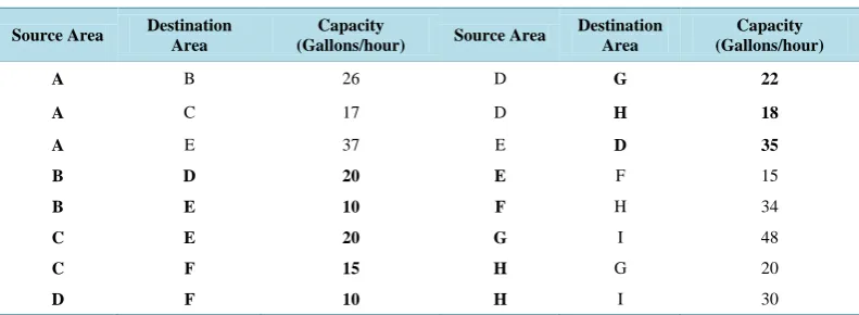
[image:3.595.116.512.254.399.2]Consider the water supply system in a Campus. The pipeline between the supply points of any two areas has a stated capacity in gallons per hour, given as a maximum flow at which water can flow through the pipe between those two areas. To supply water from the source area, A (say) to the sink area, I (say) and water passes through 7 other areas before reaching from source to sink. Suppose these 7 areas are B, C, D, E, F, G, H and pipeline between any two areas has a defined capacity. Table 1 shows the defined capacities of each pipeline between any two areas which can flow between corresponding two areas.
Table 1. Defined capacities of each pipeline between two areas.
Source Area Destination Area
Capacity
(Gallons/hour) Source Area
Destination Area
Capacity (Gallons/hour)
A B 26 D G 22
A C 17 D H 18
A E 37 E D 35
B D 20 E F 15
B E 10 F H 34
C E 20 G I 48
C F 15 H G 20
D F 10 H I 30
Calculate the maximum amount of water which can flow from A to I.
Solution of Example-1
Now the problem discussed in the Example 1 is converted into directed graph by representing areas as vertices of the graph and pipelines between any two areas as edges of the graph. The capacity of the pipeline in gallons per hour is represented as capacity of an edge in units between vertices.
Now, following correspondence between areas and vertices is used to create the graph.
Table 2. Correspondence between areas and vertices.
Area A B C D E F G H I
Vertex s 1 2 3 4 5 6 7 t
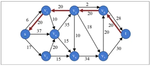
[image:3.595.193.435.590.707.2]So, the initial graph corresponding to Table 1 and Table 2 is as follows.
Now we use the modified Edmonds-Karp Method to compute a maximum flow in G.
According to the Figure 1, the maximum capacity is 48. So, the value of the variable C in the above algo-rithm will be 48.
So, 3floor(log3C) =27, this will be the value of the variable I in the 1st iteration of the algorithm.
Iteration-1: I = 27. So, the augmenting path with capacity at least 27 will be searched by the Breadth First Search (BFS) procedure. But, there is no augmenting path with capacity at least 27. So, no flow will be added to the initial flow of the graph which is 0.
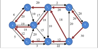
Iteration-2: I = I/3 = 27/3 = 9. So, now the augmenting path with capacity at least 9 will be searched by the same BFS procedure in the residual graph which is given in Figure 2 corresponding to the initial graph. The augmenting path will be searched till path with capacity at least 9 is found in the graph. Now, in the consecutive figures, Figure 2 shows the residual graph and Figure 3 shows the corresponding flow in the graph.
Figure 2. Residual Graph before any augmentation.
Figure 3. Flow graph after 1st augmentation.
Whenever the augmenting path is to be found in the graph, if there are more than 1 path satisfying the capaci-ty criteria, then the path is determined by BFS procedure on the basis of sequential ordering of the vertices and corresponding edges which has been given as input.
[image:4.595.188.440.596.709.2]1st Augmentation: So, the augmenting path found in 2nd iteration is s - v1 - v3 - v6 - t with capacity 20. So, the initial flow is augmented by 20 units and the flow in the graph is shown in Figure 3 giving maximum flow value f = 20. The residual graph after 1st augmentation is shown in Figure 4.
Figure 4. Residual Graph after 1st augmentation.
27 3(log 3)C=
Figure 5. Flow Graph after 2nd augmentation.
[image:5.595.217.410.268.387.2]2nd Augmentation: Now, again there is a path with capacity at least 18 and the path found in the same 2nd iteration is s - v4 - v3 - v7 - t with capacity 18. So, the maximum flow is augmented by 18 units and the flow in the graph is shown in Figure 5 giving maximum flow value f = 20 + 18 = 38. Now, there is no path with capac-ity at least 18. Same procedure will be followed until variable I becomes < 1. Residual graph after 2nd augmenta-tion is shown in Figure 6.
[image:5.595.217.411.418.525.2]Figure 6. Residual Graph after 2nd augmentation.
Figure 7. Flow Graph after 3rd augmentation.
[image:5.595.217.410.611.707.2]3rd Augmentation: Now, again there is a path with capacity at least 12 and the path found in the same 2nd ite-ration is s - v2 - v5 - v7 - t with capacity 12. So, the maximum flow is augmented by 12 units and the flow in the graph is shown in Figure 7 giving maximum flow value f = 38 + 12 = 50. Now, there is no path with capacity at least 12. Same procedure will be followed until variable I becomes < 1. Residual graph after 3rd augmentation is shown in Figure 8.
Figure 9. Flow Graph after 4th augmentation.
4th Augmentation: Now, again there is a path with capacity at least 15 and the path found in the same 2nd ite-ration is s - v4 - v5 - v7 - v6 - t with capacity 15. So, the maximum flow is augmented by 15 units and the flow in the graph is shown in Figure 9 giving maximum flow value f = 50 + 15 = 65. Now, there is no path with capac-ity at least 15. Same procedure will be followed until variable I becomes < 1.
3rd Iteration: I = I/3 = 9/3 = 3. So, now the augmenting path with capacity at least 3 will be searched in the residual graph which is given in Figure 10 corresponding to the initial graph.
5th Augmentation: So, the augmenting path found in 3rd iteration is s - v1 - v4 - v3 - v5 - v7 - v6 - t with ca-pacity 5. So, the initial flow is augmented by 5 units and the flow in the graph is shown in Figure 11 gives maximum flow value f = 65 + 5 = 70. The residual graph after 4th augmentation is shown in Figure 10.
Figure 10. Residual Graph after 4th augmentation.
Figure 11. Flow Graph after 5th augmentation.
4th Iteration: I = I/3= 3/3 = 1. So, the augmenting path with capacity at least 1 will be searched in the residual graph which is given in Figure 12 corresponding to the initial graph.
Figure 12. Residual Graph after 5th augmentation.
Figure 13. Flow graph after 6th augmentation.
[image:7.595.187.442.433.605.2]The residual graph after 6th augmentation is shown below:
Figure 14. Resulting residual network.
4.2. Example-2
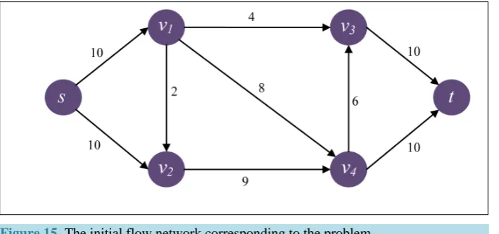
Suppose a pipeline system in a Campus to supply gas in different areas of a Campus. The pipeline between any two areas has a stated capacity in per unit per hour, given as a maximum flow at which gas can flow through the pipe between those two areas. Now, suppose we want to supply gas from the source area, suppose A to the sink area, say F and gas passes through 4 other areas before reaching from source to sink. Suppose these 4 areas are B, C, D, E and pipeline between any two areas has defined capacity.
Table 3. Defined capacities of each pipeline between two areas.
Source Area Destination Area Capacity (Gallons/hour) Source Area Destination Area Capacity (Gallons/hour)
A B 10 C E 9
A C 10 D F 10
B C 2 E D 6
B D 4 E F 10
B E 8
Calculate the maximum amount of gas which can flow from A to F.
Solution of Example-2
Now the problem discussed in the Example 2 is converted into directed graph by representing areas as vertices of the graph and pipelines between any two areas as edges of the graph. The capacity of the pipeline in unit per hour is represented as capacity of an edge in units between vertices.
Now, following correspondence between areas and vertices is used to create the graph.
Table 4. Correspondence between areas and vertices.
Area A B C D E F
Vertex S 1 2 3 4 t
[image:8.595.140.495.400.566.2]So, the initial graph corresponding to Table 3 and Table 4 is shown in Figure 15.
Figure 15. The initial flow network corresponding to the problem.
Solving the above example using our proposed algorithm, the maximum flow value f = 19.
5. Outcome
Table 5 shows a comparison of no. of iteration and no. of augmentation required to obtain the maximum flow
by using various existing methods and our proposed Modified Edmonds-Karp algorithm by means of the ab-ovetwo sample examples and it is seen that our proposed algorithm requires less number of iterations and aug-mentation paths to reach the maximum flow.
6. Conclusion
Table 5. Comparison of the resul obtained by different methods.
Name of the Algorithm Number of Iterations Number of Augmentation Example-1 Example-2 Example-1 Example-2
Ford-Fulkerson 9 6 8 5
Edmonds-Karp 7 5 7 5
Md. Al-Amin Khan et al.’s 7 5 7 5
Chintan J. & Deepak G.’s 6 4 6 3
Faruque Ahmed et al.’s 6 4 6 5
Modified Edmonds-Karp (Proposed) 4 2 6 3
sink in a flow network. We have also solved several number of maximum flow problems by using our proposed algorithm, Ford-Fulkerson algorithm, Md. Al-Amin Khan et al.’s Algorithm, and Faruque Ahmed et al.’s algo-rithm and Edmonds-Karp algoalgo-rithm to test the efficiency of the proposed algoalgo-rithm. During this process, it is observed that our proposed algorithm is faster and taking less number of iterations and less number of augmen-tations to determine the maximum flow in maximum flow problems in comparison with the other well known algorithms.
References
[1] Ford Jr., L.R. and Fulkerson D.R. (1962) Flows in Networks. Princeton University Press, Princetion, NJ.
[2] Ford, Jr. L.R. and Fulkerson D.R. (1956) Maximal Flow through a Network. Canadian Journal of Mathematics, 8, 399-404. http://dx.doi.org/10.4153/CJM-1956-045-5
[3] Edmonds, J. and Karp, R.M. (1972) Theoretical Improvements in Algorithmic Efficiency for Network Flow Problems.
Journal of the Association for Computing Machinery, 19, 248-264. http://dx.doi.org/10.1145/321694.321699
[4] Goldberg, A.V., Tardos, E. and Tarjan, R.E. (1990) Network Flow Algorithms. In: Korte, B., Lovasz, L., Promel, H.J. and Schriver, A., Eds., Paths, Flows, and VLSI-Layout,Vol. 9, Springer-Verlag, Berlin Heidelberg, 101-164.
[5] Goldberg, A.V. and Tarjan, R.E. (1988) A New Approach to the Maximum-Flow Problem. Journal of the Association for Computing Machinery, 35, 921-940. http://dx.doi.org/10.1145/48014.61051
[6] Goldberg, A.V., Plotkin, S.A. and Tardos, E. (1991) Combinatorial Algorithms for the Generalized Circulation Prob-lem. Mathematics of Operations Research, 16, 351-381. http://dx.doi.org/10.1287/moor.16.2.351
[7] Goldberg, E. and Rao, S. (1998) Beyond the Flow Decomposition Barrier. Journal of the ACM, 45, 783-797.
http://dx.doi.org/10.1145/290179.290181
[8] Cherkasky, B.V. (1977) An Algorithm for Constructing Maximal Flows in Networks with Complexity of
(
2)
O V E
Operations. Mathematical Methods of Solution of Economical Problems, 7, 117-125. (In Russian)
[9] Jain, C. and Garg, D. (2012) Improved Edmond Karps Algorithm for Network Flow Problem. International Journal of Computer Applications, 37, 48-53. http://dx.doi.org/10.5120/4576-6624
[10] Kelly, D. and O`Neill, G.M. (1991) The Minimum Cost Flow Problem and The Network Simplex Solution Method. Master of Management Science Dissertation, University College Dublin.
[11] Dinic, E.A. (1970) Algorithm for Solution of a Problem of Maximum Flow in a Network with Power Estimation. So-viet Math Doklady, 11, 1277-1280. http://www.citeulike.org/user/Fujisaki/author/Dinic:EA
[12] Goldfarb, D. and Jin, Z.Y. (1996) A Faster Combinatorial Algorithm for the Generalized Circulation Problem. Mathe-matics of Operations Research, 21, 529-539. http://dx.doi.org/10.1287/moor.21.3.529
[13] Goldfarb, D., Jin, Z.Y. and Orlin, J.B. (1997) Polynomial-Time Highest-Gain Augmenting Path Algorithms for the Generalized Circulation Problem. Mathematics of Operations Research, 22, 793-802.
http://dx.doi.org/10.1287/moor.22.4.793
[14] Hamdy, A.T. (2007) Operations Research: An Introduction. 8th Edition, Pearson Prentice Hall, Upper Saddle River, New Jersey.
[15] Mallick, J.B. (2014) An Efficient Network Flow Approach: On Development of New Idea & A Modification of EDMONDS-KARP Algorithm. M. Phil. Thesis, Department of Mathematics, Jahangirnagar University.
and System Sciences, 21, 203-217. http://dx.doi.org/10.1016/0022-0000(80)90035-5
[17] Ahmed, F., Khan, Md.A., Khan, A.R., Ahmed, S.S. and Uddin, Md.S. (2014) An Efficient Algorithm for Finding Maximum Flow in a Network-Flow. Journal of Physical Sciences, 19, 41-50.