Lancaster University Management School
Working Paper
2006/023
The process of using a forecasting support system
Paul Goodwin, Robert Fildes, Michael Lawrence and
Konstantinos Nikolopoulos
The Department of Management Science Lancaster University Management School
Lancaster LA1 4YX UK
© Paul Goodwin, Robert Fildes, Michael Lawrence and Konstantinos Nikolopoulos All rights reserved. Short sections of text, not to exceed
two paragraphs, may be quoted without explicit permission, provided that full acknowledgement is given.
The LUMS Working Papers series can be accessed at http://www.lums.lancs.ac.uk/publications/
The process of using a forecasting support system
Paul Goodwin1* Robert Fildes2,
Michael Lawrence3, Konstantinos Nikolopoulos4,
1
The Management School, University of Bath, Bath, BA2 7AY, United Kingdom.
Email: [email protected]. Tel (44) 1225 383594, Fax: (44) 1225 826473
2
Department of Management Science, Lancaster University Management School, LA1 4YX, United Kingdom.
3
School of Information Systems, Technology and Management, University of New South Wales, Sydney 2052, Australia
4
Manchester Business School, The University of Manchester, Booth Street West Manchester M15 6PB, United Kingdom
April 2006
Abstract
The actions of individual users of an experimental demand forecasting support system were traced
and analyzed. Users adopted a wide variety of strategies when choosing a statistical forecasting
method and deciding whether to apply a judgmental adjustment to its forecast. This was the case
despite the users reporting similar levels of familiarity with statistical methods. However, the
analysis also revealed that users were very consistent in the strategies that they applied across
twenty different series. In general, the study found that users did not emulate mechanical
forecasting systems in that they often did not choose the forecasting method that provided the best
fit to past data. They also tended to examine only a small number of methods before making a
selection, though they were likely to examine more methods when they perceived the series to be
difficult to forecast Individuals who were relatively unsuccessful in identifying a well fitting
statistical method tended to compensate for this by making large judgmental adjustments to the
statistical forecasts. However, this generally led to forecasts that were less accurate than those
produced by people who selected well fitting methods in the first place. These results should be of
particular interest to designers of forecasting support systems who will typically have some
stylised representation of the way that users employ their system to generate forecasts.
Key words: Judgmental forecasting, forecasting support system, forecaster behaviour, forecasting
tasks
Acknowledgements This research was supported by Engineering and Physical Sciences Research
Introduction
Almost all research into judgmental forecasting has focussed on groups of forecasters, as opposed to individuals. For example, typical research questions are "Does the use of method A lead, on average, to more accurate judgmental forecasts than method B?” (e.g. Sanders, 1997, Goodwin, 2000, Webby et al, 2005) or "Will judgmental forecasters be on average more accurate if
condition X applies in the environment rather than condition Y?” (e.g. Lawrence and Makridakis, 1989, O’Connor et al., 1993). In addition,, some studies have pooled data on individuals in order to develop models of the processes that the average forecaster adopts when making forecasts (e.g. Lawrence and O’Connor, 1992, Bolger and Harvey, 1993, Goodwin, 2005), in particular in the examination of financial analysts’ forecasts (see for example, Easterwood and Nutt, 1999). While many of these studies have produced results which are of great potential value in understanding the behaviour of forecasters and improving accuracy (Armstrong, 2001) they have also usually found that there are considerable differences between individual forecasters, in the forecasting strategies they employ and the resulting accuracy they obtain. Thus, although a particular method may, on average, improve judgmental forecasting accuracy in a particular context, there is no guarantee that it will work for a given individual. Indeed, Stewart (see: Ayton et al., 1999) has pointed out that while much research has assumed that judgment processes are universal and are independent of the individual, research should be conducted which makes the opposite assumption and fully recognises the importance of the individual.
This suggests that software designers who are responsible for producing commercial systems that support the forecasting task (forecasting support systems (FSSs)) should also consider the ways in which individuals use their systems to produce forecasts. A mismatch between the software designer’s model of how a system will be used and actual use is likely to impair the system’s functionality. However, little is known about the diversity of strategies that users adopt, the effect of these strategies on forecast accuracy and the extent to which individuals are consistent in their employment of particular strategies.
This paper describes a study that recorded all the keyboard and mouse actions of the users of a forecasting support system in order to address the following research questions:
1) How do individuals carry out the task of selecting a statistical forecasting method and what influences their propensity to apply judgmental adjustments to the resulting forecasts? 2) How much variation is there between individuals’ strategies and is this variation sufficient to justify designing systems that vary in the support that they provide to individuals?
3) Are particular strategies associated with inaccurate forecasting? 4) How consistent are individuals in applying a given strategy over time? 5) Can a broad classification of strategies be identified?
The paper is structured as follows. First other studies which have considered the implications of individual differences for decision support are reviewed. Then the forecasting task and the computerised system that was designed to support it are described. An analysis of how the subjects used the system is then used to answer the research questions. Finally the implications of this analysis for FSS design are discussed.
Individual differences and decision support
The decision support literature of the 1970s and early 1980s recognised that individuals differ in
decision support system. (e.g. Driver and Mock, 1975, Dickson et al, 1977, Bariff and Lusk, 1977
and Benbasat and Taylor, 1978). Zmud (1979) identified three main attributes of decision makers
that impacted on their use of decision support systems: cognitive style, personality and
demographic/situational variables. A key belief inherent in these papers was that the acceptability
and subsequent use of a system could be predicted from these attributes. This implied that a system
could be tailored to provide appropriate facilities that either complemented, reinforced or
attempted to correct the user’s decision making process and also improved the likelihood that the
system would be accepted in the first place. However, Huber (1983) questioned the value of using
cognitive style as a basis for system design. He argued that the literature on cognitive style lacked
both an adequate underpinning theory and reliable and valid instruments to measure cognitive
style. In the light of this Huber concluded that further research into cognitive style was unlikely to
lead to improvements in the design of systems. Nevertheless, some researchers have continued to
investigate the effect of cognitive style on DSS use. For example, Zinkhan et al (1987) considered
the effect of cognitive differentiation (together with personality, demographic and other variables)
on decision makers’ usage of, and satisfaction with, a marketing decision support system.
However, there is another approach to tailoring the response of a support system to an individual.
This does not involve using precursor variables to anticipate future use. Instead it involves directly
monitoring the actions of individuals using the system in order to identify patterns that might
signal either functional or dysfunctional use and the need for particular types of support. Such an
approach is likely to be particularly relevant for forecasting support systems because the use of
such systems usually involves carrying out similar tasks many times (thus allowing data to be
principles that provide guidance how the task should be carried out (Armstrong, 2001). For
example, the forecasting research literature indicates that forecast accuracy tends to be reduced
when a forecaster manifests a propensity to adjust statistical forecasts judgmentally, despite not
being in possession of important new information about exceptional events (Sanders and Ritzman,
2001). Whether such a pattern of actions is associated with particular cognitive styles or
personality or demographic variables is not known. Nevertheless, support mechanisms designed to
reduce the propensity (such as provision of guidance (Silver, 1991) or the requirement to record a
reason for the adjustment (Goodwin, 2000)) could still be evoked if the pattern is detected. The
rest of the paper investigates the extent to which such patterns are detectable and specific to
individual system users.
The experiment
The task and system
The experimental task was designed to replicate that found in many supply-chain based companies
where computer systems are used to obtain product demand forecasts from time series data. In
performing the task forecasters have an opportunity either to choose a statistical forecasting
method and its associated parameter values or to allow the system to identify the ‘optimum’
statistical method automatically. Note that, in many companies, these forecasts may subsequently
be modified at review meetings of managers, ostensibly to take into account market intelligence
The PC based support system was identical to the ‘high participation’ system employed by
Lawrence et al (2002). Subjects running the program first supplied answers to a questionnaire.
The subsequent screen displayed a brief explanation of the experimental task before subjects
engaged in a trial run of the program to familiarise themselves with its facilities. They then used
the FSS to estimate one-step-ahead forecasts for each of 20 monthly sales time series. Because the
focus of this study is on individual differences all the forecasters faced the same forecasting task
under the same conditions, although the time series were presented in a random sequence in order
to remove order effects. The instruction sheet told the subjects they were to act as product
managers responsible for developing a monthly forecast for 20 key products. At the conclusion of
the experiment another questionnaire was completed by the subjects.
About the subjects
The subjects were 32 management students at Lancaster University, all of whom were taking a
course in forecasting. As an incentive, monetary rewards were given to the subjects who produced
the most accurate forecasts. The subjects indicated that they had some familiarity with statistical
forecasting methods (of the type available in the FSS) and with methods of technique selection.
Their average rating on a 1 to 3 familiarity scale (1= not at all familiar, 2 = some familiarity, 3
=very familiar) was 2.2. (There was little individual variation here -only 6 subjects rated their
familiarity outside the range 2 to 2.5 on the 1 to 3 scale.) This may exceed the levels of familiarity
of forecasting personnel in many companies (Fildes and Hastings, 1994, Watson, 1996). Only a
third of the subjects made use of the five help buttons available on the FSS -these gave a brief
explanation of each forecasting method. Those that used the help facility did so on average just
Generation of the Time Series
The 20 time series were artificially generated to simulate non-seasonal demand patterns
experienced by supply chain based companies. They included: i) series without a systematic trend,
ii) series with upward or downward local linear trend, iii) series with damped trends, iv) series
with a reversal of the trend, v) random walks vi) white noise series- with step changes in the
underlying mean- and vii) irregular series. The noise associated with a given series was
independently sampled from a normal distribution with a mean of zero and a standard deviation of
either 15 or 45, yielding nine 'high noise' and eleven 'low noise' series, respectively. Graphs of two
of these series can be seen in figures 1 and 2.
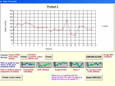
The Forecasting Support System
Figure 1 shows a typical screen display seen by subjects. The FSS presented a graph of the sales of
the product in the previous 20 months and the user had several decisions to make in order to obtain
a provisional forecast for month 21. These decisions related to the statistical forecasting method to
be used and the parameter value(s) to employ with a given method. Such choices are typically
available and exercised by company forecasters (Goodwin et al, 2006).
**Please insert figure 1 about here**
.a) Choice of forecasting method. Ten methods were available in the system: exponential
smoothing, Holt's method, damped Holt's method, Naïve 1 and an average of any two of these
methods (Makridakis et al., 1998). A brief explanation of each method, and an indication of the
mouse. Subjects had the opportunity to ask the system automatically to identify the method which
gave the closest fit (i.e. the minimum mean squared error) to the past data and to produce a
forecast using this method. Alternatively, they could choose their own method from those
available.
b) How the parameters of each method were obtained. Subjects could choose to use default
parameter values preset by the FSS, or they could ask the system to identify the parameter values
that had yielded the most accurate one-month-ahead sales forecasts over the previous 20 months. A
further choice was available here: the system could be asked to identify either the parameter values
that minimised the mean absolute error (MAE) of these previous forecasts or the values that
minimised their mean squared error (MSE). The MSE penalises large forecast errors more
severely.
When the subject had made these choices, the forecast for month 21 using the selected method was
superimposed on the sales graph, together with the method's forecasts for the previous 20 months.
At this point the subject could decide either i) to accept this forecast and move on to the next
product, ii) to make a judgmental adjustment to the forecast (using the mouse to indicate on the
graph where the adjusted forecast should be) or iii) to try out an alternative statistical method. In
the latter case, a record of the month 21 forecasts of all methods previously examined for the
current product was available at the click of a command button.
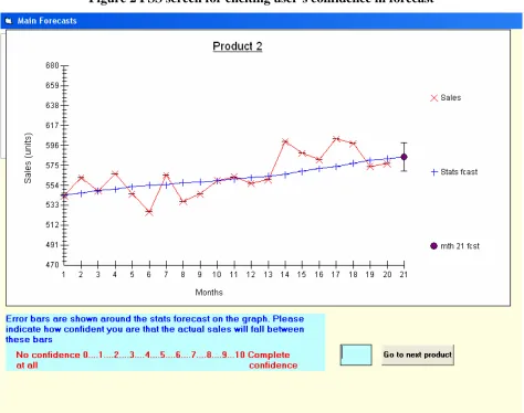
When subjects, had finally determined the forecast for a given product, the FSS displayed a
the forecast plus and minus the noise standard deviation. Subjects were then asked to indicate, on a
scale from 0 ('no confidence at all') to 10 ('complete confidence'), how confident they were that the
interval would contain the actual sales value for month 21.
**Please insert figure 2 about here**
The Questionnaires
A pre-experiment questionnaire measured subjects' familiarity with forecasting techniques and
concepts. This was presented on the computer screen and subjects used the mouse to indicate their
responses. The post-experiment questionnaire, which was also computer-based, is shown in
Appendix 1. The questions in this questionnaire were intended to elicit subjects' perceptions of the
ease of use, usefulness and trustworthiness of the FSS tool that they had just been using. The
design of the questionnaire enabled scores for the constructs 'ease of use', 'usefulness' and
'satisfaction’ using the transformations shown in Appendix 2.
The tracing method
The actions of the individuals using the program were traced by recording every key stroke and
mouse operation. The advantages of using computerised process tracing in order to develop an
understanding of how decision makers use decision support systems have been discussed by Cook
and Swain (1993). These include the unobtrusive nature of the tracing tools. To date, the method
How individuals made their forecasts
The process by which individuals used the FSS to arrive at each sales forecast can be characterised
by four features:
i) how well the forecasts of the chosen statistical forecasting method fitted the past sales data;
ii) the number of times the individual fitted a statistical method to the past sales series, before choosing the method that they thought was appropriate;
iii) whether they decided to apply a judgmental adjustment to the forecast of their chosen method;
iv) the size of any judgmental adjustment that was applied.
The fit of the chosen method's forecasts to past sales data
Most purely mechanical forecasting systems choose statistical methods, and their parameter values, on the basis of how well their forecasts fit past data. In general, there was little evidence that subjects were either able, or willing, to emulate this. An optimise button was available to indicate the best fitting method for the past 20 observations, but this was used to obtain only 14.1% of the forecasts examined and only 9.7% of the forecasting methods finally chosen (with just over 14 % of these 'optimised' forecasts subsequently judgmentally adjusted). There is evidence in the literature that the fit of a forecasting methods to past data is often only weakly correlated with the ex ante accuracy of these methods (for example Fildes and Makridakis, 1988 indicated a
to impact on demand. Choosing a method with a close fit to past data would therefore have been an appropriate strategy for most of the series.
Several of the statistical forecasts chosen were based on default parameter values (e.g. a smoothing constant of 0.1 for simple exponential smoothing), even though the graphical display showed, in many cases, that these forecasts provided a very poor fit to the past time series. For a given series, the (mean squared error) MSE of the chosen forecasting method can be compared with that of the available method offering the lowest MSE on that series. We will define the ratio of the two MSEs as the overall fit ratio.
i.e., overall fit ratio (OVR) =
system on available methods of MSE Lowest method chosen of MSE
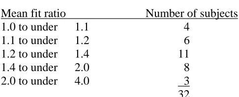
Clearly, where a subject chooses the best fitting method that is available on the FSS, for a given series, the fit ratio will be 1.0. The mean fit ratio of methods selected by subjects averaged over all twenty series was 1.44.
Nevertheless, as table 1 shows, this overall mean obscures the fact that there were considerable differences between the mean fit ratios obtained by individual subjects.
**Please insert Table 1 about here**
When subjects tried several forecasting methods for a given product they did not always select the best fitting method of those they had examined. This can be seen by considering the ratio of the fit of the chosen method to the best fitting method they saw, i.e.,
fit ratio (over methods seen) = MSE of chosen method
lowest MSE of methods examined
The mean ratio here was 1.17. Table 2 shows the variation in this ratio across the subjects
Number of methods examined
On average, the number of statistical methods that subjects examined before selecting a method was 2.6 though, as table 3 shows, there were again considerable individual differences1. Perhaps because of fatigue or increasing familiarity with the task, subjects tended to try more methods for the ten earliest series that they saw (an average of 3.2 methods per series compared to 2.0 for the second ten seen, t = 4.43. p <0.001). However, because the product series were presented to subjects in random order this did not have any effect on the forecasts of particular series (the correlation between the mean position in which the series was displayed (1= first series displayed, 20 = last) and the number of methods tried was only -0. 055).
**Please insert table 3 about here**
The number of statistical forecasting methods tried by subjects varied significantly across the 20
series. The hypothesis that the number of methods tried was uniformly distributed across the series
was rejected at p <0.001 (Χ219 = 55.6). Why did subjects try out more methods on some series than
others? One possibility is the difficulty of modelling the patterns of particular series -the more
difficult the pattern, the more methods people will try. The MSE of the 'optimal' available method
was used as a proxy for the difficulty of modelling the pattern and this was significantly correlated
with the number of methods tried (r = 0.46, p<0.05). However, the levels of sales in the different
series varied considerably so that they appeared on graphs with different vertical scales. As a result
a forecast error of 10 units in one series might appear to subjects to represent a larger gap than an
error of 100 units in another series. To take this into account, for each series the MSE of the
minimum) so that the resulting measure reflected the lack of fit of the statistical forecast as it might
be perceived by the subjects. As hypothesised, this led to a higher correlation with the number of
methods tried (r= 0.56, p<0.01). Thus, although subjects in general did not tend to choose the best
fitting methods, the perceived lack of fit of the methods they tried may have spurred them on to try
further methods2.
Consequences of trying more methods
In general, series which had more statistical methods applied to them were forecasted less
accurately (the correlation between number of methods tried and the mean absolute percentage
error (MAPE) of the chosen statistical forecast was 0.46, p<0.05 while the correlation with the
MAPE of the final -possibly judgmentally adjusted-forecast was 0.47, p<0.05). This is perhaps not
surprising as the above analysis suggests that more methods were tried on the more
difficult-to-forecast series.
Did people who tried more forecasting methods than their fellow subjects obtain more accurate
final forecasts? In general, the answer was 'no' -the correlation between the total number of
methods subjects tried and the MAPE of their chosen statistical forecasts was -0.005, while the
correlation between the number of methods and the final (possibly judgmentally adjusted)
forecasts was 0.192. Did trying more methods lead to a mean overall fit ratio closer to 1.0? There
was no evidence for this (r= 0.12). Nor was their any evidence that subjects who tried more
1
This figure includes times when subjects revisited a method that they had already tried on a given series
2
methods, adjusted fewer forecasts (r = -0.164) or that they were more confident in their final
forecasts (r = 0.159). However, it is important to note that these correlations also mask some
interesting differences between subjects which will be explored later.
Adjustment behaviour
Why do subjects decide to apply a judgmental adjustment to particular statistical forecasts, while
leaving other forecasts unadjusted? This can be investigated both in terms of the characteristics of
the different series and also in relation to the behaviour of the different subjects.
There was no significant difference in the number of adjustments applied to the 20 different series
(Χ219 = 9.89, not significant), suggesting that propensity to adjust could not be explained by the
characteristics of particular series. Many judgmental adjustments made by subjects were relatively
small -half of the absolute percentage adjustments were below 2.26%. However, subjects who
chose statistical forecasts that provided relatively poor fits to the past observations did tend to
adjust their forecasts more often and make bigger adjustments. The correlation between the mean
'overall' fit ratio of the forecasting methods chosen by subjects and the number of adjustments they
applied was 0.467 (p< 0.01), while the correlation between subjects' mean 'overall' fit ratios and
their mean absolute percentage adjustments (MAPA) was 0.638 (p<0.001)3. All of this suggests
that subjects who could only obtain poorly fitting statistical methods recognised the inadequacy of
their forecasts and tried to compensate by applying judgmental adjustments to them. There is some
and the complexity of the series measured on a scale using a score of 1 for a 'flat' underlying pattern, 2 for a trend and 3 for an erratic underlying pattern. All of these variables yielded correlations that were close to 0.
3
evidence from the literature that judgmental forecasters can recognise forecasts that are in need of
adjustment, even when they only have access to time series information (Willemain, 1989)
Other factors that might have explained the propensity to adjust forecasts did not yield significant
associations. For example, before starting the experiment, subjects were asked to indicate (on a
five-point scale) their strength of agreement with the statement that "statistical forecasts are less
important than human judgment". The correlation between their strength of agreement with this
statement and the number of judgmental adjustments they made was only 0.026.
Consequences of adjustments and lack of fit
To investigate the effect of the size of the adjustments and the overall fit ratio on forecast accuracy
the following multiple regression model was fitted to the data
MAPE =5.21 + 1.29 OVR + 0.714 MAPA - 0.307 (OVR x MAPA) (0.000 (0.066) (0.009) (0.036))
R-squared = 28.1%
where OVR = the overall fit ratio of their selected statistical method compared to the best method
and MAPA is the mean absolute percentage adjustment.
p-values for the regression coefficients are shown in brackets,.
Shown below are some predictions of the model for four combinations of overall fit ratios
Overall Fit ratio MAPA Predicted MAPE
1,0 0% 6.5%
1.0 1% 6.9%
2.0 0% 7.8%
2.0 5% 8.3%
These predictions indicate that judgmental adjustments tended to reduce accuracy. While this is
perhaps not surprising when the adjustment were applied to well-fitting methods, the predictions
also show that making large adjustments to poorly fitting methods also tended to reduce accuracy.
Thus it appears that subjects who attempted to compensate for poor fitting forecasting methods by
making relatively large judgmentally adjustments to their forecasts tended to be less accurate than
those who obtained well fitting methods, in the first place, and made no (or very minor)
adjustments.
Other points
Interestingly, subjects who spent a larger percentage of their total time on the trial run tended to
achieve more accurate forecasts. The correlation between the % of time on the trial run and the
MAPE was -0.435 (p<0.02). Similarly, the correlation between the actual time spend on the trial
run and the MAPE was -0.365 (p<0.05). This may reflect the commitment of the individual
subjects or it may indicate that time spent exploring and practising using an FSS is beneficial.
MAPEs achieved by subjects were very small and not significant. Performance was therefore not associated with the extent to which the FSS was regarded as "easy to use" and "useful". It is particularly noteworthy that subjects' perception of their performance bore no relationship with the actual forecasting accuracy that they achieved (r = 0.051).
Were the forecasters consistent?
How consistent were subjects in applying particular strategies? As indicated earlier, consistency
would be necessary for an FSS to recognise particular individual traits so that appropriate guidance
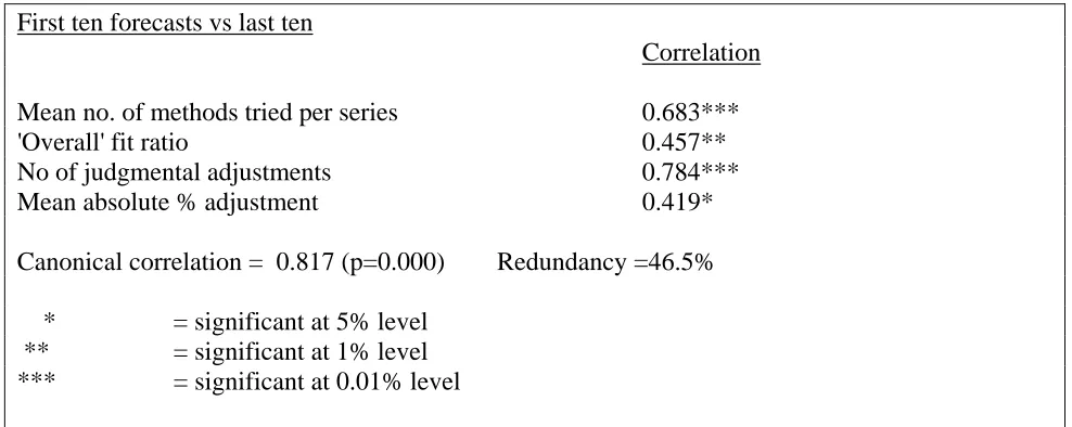
could be provided. Table 4 shows the correlations between the characteristics of individuals’
strategies for the first ten and last ten series that they forecast. These correlations indicate high
levels of consistency, particularly for the mean number of forecasting methods that were examined
for each series and for the frequency with which judgmental adjustments were made. The high
value of the canonical correlation coefficient, which reflects the correlation across all four
characteristics in table 4, is also indicative of consistency.
**Please insert Table 4 about here**
An interesting question relates to how many forecasts an FSS would need to record before the characteristics of an individual strategy could be discerned. Table 5 suggests that reasonable predictions of an individual’s strategy can be based on as few as five forecasts and that even a prediction based on only one forecast has some value.
Characterising Forecaster Behaviour: Analysis of subjects by sub-groups
particular, this allows the effects of interactions of features of these strategies to be studied. For example, in general there may be no relationship between the number of statistical methods tried and the accuracy of the resulting forecasts. However, for some subjects trying a large number of methods may be an essential part of an effective forecasting strategy in that it used to explore and gain insights into the forecasting problem before making a commitment to a forecast. In other cases trying a large number of methods be may symptomatic of 'thrashing around' in desperation in an attempt to find an acceptable model. Cluster analysis, using Ward’s method followed by k-means clustering was used to group the subjects according to five variables: the number of methods they tried on the series the mean 'overall' fit ratio of the method they finally chose, the number of judgmental adjustments they made, their mean absolute percentage adjustment
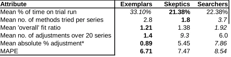
(averaged over occasions when they adjusted) and the total time they spent on the task, including the trial run .The variables were standardized and, as recommended for example by Sharma, (1996), several other clustering methods were also used and the results compared. One subject would not fit easily into any of the clusters and was removed from the analysis; this demonstrates the difficulty of trying to find a categorization of user types that includes all possible users. From this cluster analysis, three groups were identified and, for ease of reference, names assigned to them. These groups are described below and the data relating to them is summarised in table 6.
Group 1: "The Exemplars"
Fifty-five percent of subjects (excluding the outlier) were assigned to this group who achieved the most accurate forecasts. Table 6 shows that they had the ’best’ mean overall’ fit ratio, made the fewest adjustments and, when they adjusted, they made the smallest absolute percentage adjustments. Interestingly, this group spent the largest percentage of the total time using the FSS on the trial run where they were able to learn about the support system’s facilities.
Group 2: "The Sceptics"
judgmental adjustments which were, on average, relatively large. The result of all of this was that their ‘final’ forecasts were less accurate than those of Group 1.
Group 3: “The Searchers”
This relatively small group (16% of subjects) produced the least accurate forecasts. Despite exploring the largest number of forecasting methods per series in a search for an appropriate method they achieved the ‘poorest’ overall mean fit ratio and made the largest, judgmental
adjustments to their statistical forecasts. There was evidence that these forecasters tended to ‘cycle’ between forecasting methods –often returning several times to methods that they had already investigated. Oddly this group had a significantly higher level of disagreement (p=0.002) than the other groups with the statement: “Statistical forecasts are less important than human judgment”
**Please insert Table 5 about here**
**Please insert table 6 about here**
Surprisingly, there were no significant differences between the three groups in their saistifaction with the FSS or in their ratings of its ease of use and usefulness.
Conclusions
This study has shown that there can be considerable variation in the approaches people adopt when using a forecasting support system (FSS). This can occur even where these people indicate that they have similar levels of familiarity with the methods available in the system.
adjustment tends to lead to forecasts that are less accurate than those produced by people who select well fitting methods in the first place.
A key result of the study is that users were consistent in their approach throughout the twenty forecasts they made (subject to a general tendency to try fewer methods as time went on). This suggests that adaptive FSSs could be designed to recognise particular strategies at an early stage, enabling the interface to adapt to the particular needs, strengths and weaknesses of these users. For example, the system could highlight information that was being insufficiently taken into account (such as the lack of fit of the chosen forecasting method or its inability to deal with a trend in the series) and also guide the user towards the selection of more appropriate methods.
Interestingly, people who devoted a larger percentage of their time familiarising themselves with the FSS on a trial set of data, tended to achieve more accurate forecasts.
The study has also provided some evidence that the behaviour of sub-groups of forecasters can be identified. This behaviour ranged from people who were able to produce accurate forecasts after examining very few methods to those who examined many methods and yet only obtained relatively inaccurate forecasts. Analysis by sub-group allowed interaction between elements of behaviour to be taken into account. It also permits us to identify good forecasting strategies. For example improved accuracy can be obtained by:
• spending time familiarising oneself with the system and then examining only a few
forecasting methods and
• choosing a method which provided a good fit to past data,
and then
• avoiding making substantial judgmental adjustments
of familiarity with forecasting processes and an identical level of experience in using the system. Moreover, clustering individuals into sub-groups can be sensitive to the methodological choices made during the application of cluster analysis (e.g. Ketchen and Shook, 1996) and, as we found here, there may be some individuals who do not easily conform to any group.
While the results of this study should be of value to those designing FSSs the extent to which
inferences can be drawn from them may be constrained the fact that this was a laboratory study
involving management students. Although researchers like Remus (1986) have indicated that
student subjects can act as good surrogates for managers in experiments the laboratory
environment of this study has meant that the acceptability and use of the system under working
Appendix 1 Questionnaires
Pre-experiment questionnaire
Please indicate your strength of agreement with the following statements. Indicate your answer to
each question by using the mouse to click on one of the five numbers which seems to match your
feelings.
Q1 In developing ROUTINE forecasts the computer can probably be allowed to function with little manual intervention.
strongly agree 1………2………3………4………5 strongly disagree
Q2 In developing IMPORTANT forecasts I would expect that even most good computer-based forecasts would need to be modified manually
strongly agree 1………2………3………4………5 strongly disagree
Q3 Statistical forecasts are less important than human judgment
strongly agree 1………2………3………4………5 strongly disagree
Q4 People are generally biased in their judgments
strongly agree 1………2………3………4………5 strongly disagree
Q5 It is important to use statistical forecasts to remove subjectivity
Please rate your familiarity with the following forecasting techniques and concepts
Not at all Some Very familiar familiarity familiar
Exponential Smoothing 1……….2……….3
Holt-Winters 1……….2……….3
Combining Forecasts 1……….2……….3
Forecast Technique Selection 1……….2……….3
Post-experiment questionnaire
Please indicate your thoughts about the forecasting system you have just been using. Indicate your answer to each question by using the mouse to click on one of the five numbers which seems to match your feelings.
A I consider the system producing the computer forecast advice to be:
1. accurate 1………2………3………4………5 not accurate
2. useless 1………2………3………4………5 useful
3. not helpful 1………2………3………4………5 helpful
4. in need of little in need of much manual intervention 1………2………3………4………5 manual intervention
5. trustworthy 1………2………3………4………5 untrustworthy
6. easy to use 1………2………3………4………5 hard to use
I consider the system producing the computer forecast advice to be:
7. responsive 1………2………3………4………5 unresponsive
8. uninformative 1………2………3………4………5 informative
9. satisfactory 1………2………3………4………5 unsatisfactory
10. inflexible 1………2………3………4………5 flexible
adaptive not adaptive to 11. to requirements 1………2………3………4………5 requirements
I consider the system producing the computer advice to be:
12. not amenable to amenable to
easy intervention 1………2………3………4………5 easy
intervention
13. clear and not clear
comprehensible 1………2………3………4………5 and
comprehensible
14. sufficiently under not sufficiently
under my control 1………2………3………4………5 under my control
B How do you feel about your performance?
1. happy 1………2………3………4………5 unhappy
2. dissatisfied 1………2………3………4………5 satisfied
3. did as well as could have done I could 1………2………3………4………5 better
C Do you feel that you could have improved your forecast accuracy by: Click ONE box
1. trusting the computer more?
2. trusting the computer less?
3. I think I got it about right
D Taken as a whole, the overall system led to final forecasts such that I feel
1 I am comfortable I am uncomfortable with them -they with them -they do correspond to my not correspond to real beliefs 1………2………3………4………5 my real beliefs
Appendix 2. Transformations
QA1 refers to the subject's response, on the 1 to 5 scale, to question A1:
Ease of use = (-QA4 - QA6 - QA7 + QA10 - QA11 + QA12 - QA13 - QA14 + 36)/8
Usefulness = (-QA1 + QA2 + QA3 - QA5 + QA8 - QA9 + 18)/6
Satisfaction = (- QB1 + QB2 - QB3 - QD1 + QD2 + QC + 18)/6
where, for question C, the selection of options C1, C2 and C3 generated values of 5, 1 and 3 for
References
Armstrong, J.S. (2001). Principles of Forecasting, Boston: Kluwer Academic Publishers.
Ayton, P, Ferrell, W.R. & Stewart, T.R. (1999). Commentaries on "The Delphi technique as a forecasting tool: issues and analysis" by Rowe and Wright, International Journal of Forecasting, 15, 377-381.
Bariff, M.L. & Lusk, E.G. (1977.) Cognitive and personality tests for the design of management information systems, Management Science, 23, 820-829.
Benbasat, I. & Taylor, R.N. (1978). The impact of cognitive styles on information system design,
MIS Quarterly, 2, 43-54.
Bolger, F., & Harvey, N. (1993). Context-sensitive heuristics in statistical reasoning, Quarterly Journal of Experimental Psychology, 46A, 779-811.
Cook, G.J., & Swain, M.R. (1993). A computerized approach to decision-process tracing for decision support system design, Decision Sciences, 24, 931-952.
Dickson, G.W., Senn, J.A. & Chervany, N.L. (1977). Research in management information systems: the Minnesota experiments, Management Science, 9, 913-923.
Driver, M.J. & Mock, T.J. (1975). Human information processing. Decision style theory and accounting information systems, Accounting Review, 50, 490-508.
Easterwood, J.C. & Nutt, S.R. (1999). Inefficient in analysts’ earnings forecasts: systematic miseaction systematic optimism. Journal of Finance 54, 1777-1797.
Fildes R., & Hastings, R. (1994). The organisation and improvement of market forecasting.
Journal of the Operational Research Society, 45, 1-16.
Goodwin, P. (2000). Improving the voluntary integration of statistical forecasts and judgment,
International Journal of Forecasting,16, 85-99.
Goodwin, P. (2005). Providing support for decisions based on time series information under conditions of asymmetric loss. European Journal of Operational Research, 163(2), 388-402.
Goodwin., P., Lee, W. Y., Fildes, R., Nikolopoulos, K. & Lawrence, M. (2006). Understanding the Use of Forecasting Software: an Interpretive study in a Supply-Chain Company, University of Bath Management School Working paper.
Huber, G.P. (1983). Cognitive style as a basis for MIS and DSS: Much ado about nothing?
Management Science, 29, 567-579.
Ketchen, D.J. & Shook, C.L. (1996). The application of cluster analysis in strategic management research: an analysis and critique, Strategic Management Journal, 17, 441-458.
Lawrence, M., Goodwin, P. & Fildes, R. (2002). Influence of user participation on DSS use and decision accuracy. Omega, International Journal of Management Science., 30, 381-392.
Lawrence, M.J. , & Makridakis, S. (1989). Factors affecting judgmental forecasts and confidence intervals, Organizational Behavior and Human Decision Processes, 42, 172-187.
Lawrence, M.J. , & O'Connor, M.J.(1992). Exploring judgemental forecasting, International Journal of Forecasting 8, 15-26.
Makridakis, S., Wheelwright, S.C. & Hyndman, R.J.(1998). Forecasting. Methods and Applications 3rd edition, Chichester: Wiley.
O'Connor, M., Remus, W., & Griggs, K. (1993). Judgemental forecasting in times of change,
International Journal of Forecasting, 9, 163-172.
Remus, W. (1986). Graduate Students as Surrogates for Managers in Experiments on Business Decision Making. Journal of Business Research,14, 19-25.
Sanders N.R. (1997). The impact of task properties feedback on time series judgemental forecasting tasks Omega, 25, 135-144.
Sanders, N. R & Ritzman , L.P. (2001). Judgmental adjustment of statistical forecasts, In: J.S. Armstrong (Ed.) Principles of Forecasting, Boston.: Kluwer Academic Publishers, 405-416.
Sauter, V. L. (1997). Decision Support Systems: An Applied Managerial Approach, New York :Wiley.
Sharma, S. (1996). Applied Multivariate Techniques, New York: Wiley.
Silver, M.S., (1991) Decisional guidance for computer-based support, MIS Quarterly, 15, 105-133.
Watson, M. (1996). Forecasting in the Scottish electronics industry, International Journal of Forecasting, 12, 361-371.
Webby, R. O’Connor, M. & Edmundson, B. (2005). Forecasting support systems for the incorporation of event information: an empirical investigation, International Journal of Forecasting, 21, 411-423.
Willemain, T.R.. (1989). Graphical adjustment of statistical forecasts, International Journal of Forecasting, 5, 179-185.
Zmud, R.W. (1979). Individual differences and MIS success: a review of the empirical literature,
Table 1 Mean fit ratio
Mean fit ratio Number of subjects 1.0 to under 1.1 4
1.1 to under 1.2 6 1.2 to under 1.4 11 1.4 to under 2.0 8 2.0 to under 4.0 3 32
Table 2 Mean fit ratio (over methods seen)
Mean fit ratio (over methods seen) Number of subjects
1.0 4
1.01 to under 1.10 10 1.10 to under 1.20 8 1.20 to under 1.30 3 1.30 to under 1.70 4
29* (*3 subjects never considered more than one method)
Table 3 Mean number of methods tried per series
Mean no. of methods tried per series Number of subjects
1.0 3
1.1 to under 2.0 10
2.0 to under 3.0 6 3.0 to under 5.0 10
5.0 or more 3
Table 4 Consistency
First ten forecasts vs last ten
Correlation
Mean no. of methods tried per series 0.683***
'Overall' fit ratio 0.457**
No of judgmental adjustments 0.784*** Mean absolute % adjustment 0.419*
Canonical correlation = 0.817 (p=0.000) Redundancy =46.5%
* = significant at 5% level ** = significant at 1% level *** = significant at 0.01% level
Table 5 Predicting an individual’s strategy from early forecasting behaviour
First five forecasts vs last ten
Correlation
Mean no. of methods tried per series 0.606***
'Overall' fit ratio 0.421*
No of judgmental adjustments 0.628*** Mean absolute % adjustment 0.263 (ns)
Canonical correlation = 0.758 (p=0.000) Redundancy = 37.2%
First forecast vs last ten
Correlation
No. of methods tried per series 0.401*
'Overall' fit ratio 0.384*
No of judgmental adjustments # 0.531* Mean absolute % adjustment 0.395*
(# can only be 0 or 1 for first forecast)
Canonical correlation = 0.689 (p=0.011) Redundancy = 27.4%
Table 6 Characteristic of the three groups of forecasters
Attribute Exemplars Skeptics Searchers
Mean % of time on trial run 33.10% 21.38% 22.38%
Mean no. of methods tried per series 2.8 1.8 3.7
Mean 'overall' fit ratio 1.21 1.38 1.92
Mean no. of adjustments over 20 series 1.4 9.3 6.0
Mean absolute % adjustment* 0.89 5.45 7.86
MAPE 6.71 7.47 8.54
Bold = 'smallest', Italics= 'largest'
*= averaged only over forecasts where an adjustment was made