http://dx.doi.org/10.4236/jmf.2014.41005
Game Russian Options for Double Exponential
Jump Diffusion Processes
Atsuo Suzuki1*, Katsushige Sawaki2
1
Meijo University, Gifu, Japan 2
Aoyama Gakuin University, Sagamihara, Japan Email: *[email protected], [email protected]
Received November 8, 2013; revised December 11, 2013; accepted December 27,2013
Copyright © 2014 Atsuo Suzuki, Katsushige Sawaki. This is an open access article distributed under the Creative Commons Attribu-tion License, which permits unrestricted use, distribuAttribu-tion, and reproducAttribu-tion in any medium, provided the original work is properly cited. In accordance of the Creative Commons Attribution License all Copyrights © 2014 are reserved for SCIRP and the owner of the intellectual property Atsuo Suzuki, Katsushige Sawaki. All Copyright © 2014 are guarded by law and by SCIRP as a guardian.
ABSTRACT
In this paper, we deal with the valuation of Game Russian option with jumps, which is a contract that the seller and the buyer have both the rights to cancel and to exercise it at any time, respectively. This model can be for-mulated as a coupled optimal stopping problem. First, we discuss the pricing model with jumps when the stock pays dividends continuously. Secondly, we derive the value function of Game Russian options and investigate properties of optimal boundaries of the buyer. Finally, some numerical results are presented to demonstrate analytical properties of the value function.
KEYWORDS
Stochastic Process; Game Russian Option; Double Exponential Distribution; Optimal Stopping; Optimal Boundaries
1. Introduction
Russian option was introduced by Shepp and Shiryaev [1,2] and it was one of perpetual American lookback op-tions. In Russian option, the buyer has the right to exercise it at any time. On the other hand, in Game Russian option, not only the buyer but also the seller has the right to cancel it at any time. This option is based on Game option introduced by Kifer [3]. Game option frame work can be applied to various American-type options. Therefore, we apply this frame work to Russian option. The valuation of Game Russian option can be formu-lated as a coupled optimal stopping problem. See Cvitanic and Karatzas [4], Kifer [3].
Kyprianou [5] derived the closed-form solution in the case where the dividend rate is zero. Suzuki and Sawaki [6] gave the pricing formula with positive dividend. Kou and Wang [7] presented the closed-form for the value function of perpetual American put options without dividend and so on. Suzuki and Sawaki [8] studied the pric-ing formula of Russian option for double exponential jump diffusion processes.
In this paper, we deal with Game Russian options. Game Russian option is a contact that the seller and the buyer have the rights to cancel and to exercise it at any time, respectively. We present the pricing formula of Game Russian options for double exponential jump diffusion processes. The pricing of such an option can be formulated as a coupled optimal stopping problem which is analyzed as Dynkin game. We derive the value function of Game Russian option and its optimal boundaries. Also some numerical results are presented to demonstrate analytical sensitivities of the value function with respect to parameters.
This paper is organized as follows. In Section 2, we introduce a pricing model of Game Russian options by means of a coupled optimal stopping problem given by Kifer [3]. Section 3 presents the value function of Game Russian options for double exponential jump diffusion processes. Section 4 presents numerical examples to
ify analytical results. We end the paper with some concluding remarks and future work.
2. Pricing Model
In this section, we consider the pricing model for Game Russian option. Let B t
be the process of the riskless asset price at time t defined by B t
B
0 ert, where is the positive interest rate. Let be a stan-dard Brownian motion andr W t
N t be a Poisson process with the intensity . Let Ji denote i.i.d. positive
random variables. YilogJi has a double exponential distribution and its density function is given by
1 2 1e 1 0 2e 1 0
y y
y y
f y p q ,
where 1> 1,2> 0 and 0p q, 1 such that p q 1. Under a risk-neutral probability, the process of the
risky asset price S t
at time satisfies the stochastic differential equation t
1
d
d d d 1
N t i i
S t
t W t J
S t
, (1)where and > 0 are constants. Define another probability measure P as
2d 1
exp , ,
d 2
t
P r
bW t b t b
P
d
where d
<r is a nonnegative continuous dividend rate of the risky asset,
t W
s ,N s s
, t J,
i is the information available at time t and
1 21 2
1 1
1 1
i
p q
E J
.
By Girsanov’s theorem, W t
W t
bt is a Brownian motion with respect to P. We can rewrite (1) as
1
d
d d 1 . (2)
N t i i
S t
r d t W t d J
S t
Solving (2) gives S t
S
0 expX t
, where
2
1
1
. 2
N t i i
X t r d t W t Y
Let V v
be a function of class C2. Then the infinitesimal generator of the process S t
is given by
1 2 2
e d
2
y
V v v V v r d vV v V v V v f y y
for all v> 0.
Next we introduce the four real numbers 1, 2, 3, 4. Kou and Wang [9] showed that the equation
G for all > 0 has the solutions 1, ,2 3,4, where
2 2 2 1 21 2
1 1
1 .
2 2
p q
G r d
And the four solutions satisfy the following inequalities
1 1 2 3 2 4
0 < < < <, 0 < < < <.
Remark 2.1 When the dividend rate d0, 11.
Define the process
0
max ,sup , 0 , 1.
u t
t vs S u S t S s v
Then the value function of Russian option is given by
sup e
0R
V v E v
,
where the supremum is taken for all stopping times .
Theorem 2.1 (Suzuki and Sawaki [8]) The value function VR
v of Russian option with jump is given by
1
2
3
1 1 1 1
1
, 1
, .
R
4
1
A v v B v v C v v D v v
V v
v v
v v
v
The coefficients are determined by
1
4
2 3 2 4 4 3
1 1 1
1 1
1 3 2 1 1 1 4
1 1
1
v
A v v Dv
1
2
4
1 3 1 4 4 3
2 1 1
1 1
2 1 2 3 1 1 4
1 1
1
v
B v v Dv
1
3
4
1 3 1 1 2 1 4 2 4
1 1
1 3 2 3 1 1 4
1 1
1
v
C v v Dv
1
and
1
1
1
12 1 2 2 2 3 2 4
0.
A v B v C v D v
Moreover, the optimal boundary v1 is the solution in
1,
to the equation
1
2
3
4 0A v B v C v D v
and the optimal stopping time is given by
1
inf t 0 .t v
3. Game Russian Options
Let denote a cancel time for the seller and an exercise time for the buyer. If the seller cancels the con-tract, the buyer receives
from the seller. We can think of > 0 as the penalty cost for the cancel-lation. On the other hand, if the buyer exercises it, (s)he receives
from the seller. Therefore, the payoff function for the buyer is given by
1 <
1.Let 0, denote the set of all stopping times with values in the interval
0, . Then the value functionof Game Russian option is defined by
V v
0, 0,
, , ,
sup inf
V v J v
(3)
where
, , e 1 1 0 , 0.
J v E v
And the function V
v satisfies the inequalities
,vV v v
which provides the lower and the upper bounds for the value function of Game Russian option. We define two sets A and B as
A vR V v v
.B vR V v v
A and are called the seller’s cancellation region and the buyer’s exercise region, respectively. Then the two optimal stopping times are given by
B
inf 0 ,
A t t
inf 0 .
B t t
B
Then for any v, ˆ A and ˆ B attain the infimum and supremum in (3), i.e., we have
ˆ ˆ, ,V v J
ˆ
v .
The pair
ˆ , is the saddle point of J
, ,v
.
t
0 v 1
Remark 3.1 The seller minimizes the payoff function and . From this, it follows that the seller’s optimal cancellation region is {1}.
Lemma 3.1 Suppose that 1 2
2
r d > 0. Then the function V
v is Lipschitz continuous and itsRadon-Nikodym derivative satisfies
d0 1,
d
V v
a e v v
. . . (4)
Proof. Since ˆ ˆ, and
t depend on the initial value v, we write them as ˆv,ˆvand
t v, . Re-placing the optimal stopping times ˆvby another stopping time ˆu
, we get the inequalities
v J
ˆu,ˆ , V
u
ˆu,ˆv,u
.
Note that
fo z z,V
1 2 1 2
z z z z r any
J,
v
v
1 2R. For any v>u, we have
v V
u
ˆ ˆ
ˆ ˆ 1
ˆ ˆ 1
0
ˆ ,ˆ , ˆ ,ˆ ,
ˆ ˆ ˆ ˆ
e , ,
ˆ ˆ
e sup
ˆ ˆ
e
,
u v
u v
u v
u v u v
u v u v
u v
u u
u v
V
J v J u
E v u
E H v H u H
v u E H
v u
supwhere H t
expX
t . Therefore, we obtain
0 V v V u 1.
v u
This means that V
v is Lipschitz continuous and satisfies (4).If the penalty is large enough, the seller never cancels. It is of interest to show how much should
be r neve
t
delta large for the selle r to cancel.
Lemma 3.2 Se VR
1 1
. If the penalty > , the seller never cancels. In other word me Rus-sian option is reduced to RusRus-sian option
s, Ga .
he function
Proof. Consider t U
v VR
v v . Since it holds U v
0 by Lemma 3.1 and
1 0U , we have VR
v <v . Hence, it follows that V
v <
v because the inequality
v VR
v
holds.
V
We assume that p1 and s that the jump occurs only is very useful to analyse
manageme
0
q . It mean upward. This
stochastic cash nt pr for jump diffusion processes (See Sato and Suzuki [10]). Then we can ex-pr
oblem ess G
as
2 2 2 11
1 1
1
2 2
G r d
and the equation G
has three solutions 1, 2,4, which satisfy1 1 4
1 < <2<, 0 < <. We introduce the function for 0
0 e > 1 x
v
1 2 40 0
, 1
, .
Av Bv Cv v v
V v
v v
v
and V v
V
ex V xˆ
ex0.ex
v
We set . In what follows, we determine the coefficients A B C, , and
In order t are the conditions. By value ma
e
o determine the coefficients, we prep tching condition, we have
1 0 2 0 4 0 0
e x e x e x
A B C x
and by smooth pasting condition, we have
1 0 2 0 4 0 0.
1e 2e 4e e
x x x x
A B C
of the process X t
L given by
We can get the last condition by using the infinitesimal generator
1 2
1 2
ˆ ˆ ˆ ˆ ˆ ˆ d
2 2
V x V x r d V x
V x y V x f y y
for all . For
> 0
x x<x0, we obtain
0 1 ex x y
2 4 1 1
0
1 2 4
0
1 0 1 0 2 0 4 0
1 1
0
1
1 1 1 2 1 4
1
1 1 1 2 1 4 1
ˆ d
e e e d e e d
e e e
e
e e e e .
1
x x y x y y x y y
x x
x x x
x
x x x x x
V x y f y y
A B C y y
A B C
A B C
From this, we obtain
1 2 41 2 4
1 0 1 0
2 2 2 2
1 1 2 2
2 2
4 4
1 2 4
1
1 1 1
ˆ ˆ
1
x
e 1 e 1 1
2 2 2 2
1 1 ˆ ˆ
e d
2 2
e e e
e e
x
x
x x x
x x x
L r V x
A r d B r d
C r d V x y f y y r V x
A g B g C g
A B p
02 0 4 0
2 1 4 1
e
e e ,
1
x
x C x
where g x
G
x r. By Lemma 2.1 in Kou and Wang [9], we have g
1 g
2 g
4
0. Sinceholds, we get the condition
Lr V x
ˆ 00
1 0 2 0 4 0
e x e x e x
A B C
1 1 1
2 1 4 1
e 0. 1 x
(6)
Lemma 3.3 Solvin
g the following equations
1 0 2 0 4 0 0
1 0 2 0
1e 2e
x
A B 4 0 0
0
1 0 2 0 4 0
4
1 1 1 2 1 4 1
e e e e
e e
e
e e e
1
x x x x
x x x
x
x x x
A B C
C
A B C
gives the solutions
1 0 2 0 4 0 11 1 2 4
1 1 4 2 1
1
2 1 1 4
1 2 4 2 1
1
1 4 2 1
1 1 4 2 4
, we denote them as A x
0 ,B x0, ,
A B C depend on x0
Since the coefficients and C x
0 . The number0
0 e
x
v given by (5) satisfies the equation
1 0
2 0
4 00 e 0 e 0 e
x x x
A x B x C x 1.
4. Main Theorem
Theorem 4.1 Let V
v denote the value function of Game Russian option. If , the value function is equal to the one of Russian option, i.e. V
v VR
v
then V
v. If < , is given by
2
0 0
1 4
0
0
, 1
,
0
A v v B v v C v v
V v
v v
v v
v
(7)
and the optimal stopping times are given by
ˆ inf t 0 1 ,t
0
ˆ inf 0 t v .
t
The optimal boundary v0 for the buyer is the unique solution to the equation
1.A v B v C v
In order to prove the above theorem, we need the following lemmas.
Lemma 4.1 Assume that a function V v has the following properties
; 1) V v
v and
r V v
0, for v>v0.2) It holds
r V v
0 and V v
satisfies v<V v
<v for . 3) At0
1 <v<v
0
0
unV v V v
0
vv we have .
holds. The optimal ex-ercise reg
Then, V is the value f ction of Game Russian options with dividend, i.e., V
ion is the interval
and the optimal cancellation region isV
0,
v
1 .Proof. Ito’s formul
(8)
By a, we have
e t martingale with 0 e
V t V t
0
t u
d .r V u u
Set
0
ˆ inf t 0; t 1 , ˆ inf t 0; t v,
and t ˆ ˆ. Since
r V
u
0 a.s. for u<t, we have
0e d 0
t u
r V u u
a.s. There-fore, taking expectation of (8), we have
ˆ ˆ
ˆ ˆ
e 0
V v E V v. It holds
ˆ ˆ
ˆ 1ˆ ˆ
ˆ
1ˆ ˆV . erefore w V
v J
ˆ ˆ, ,v
.Th e get
r V v
0For any , set t ˆ . The term o df u is nonpositive a.s. because . Taking expecta-tion of (8), we get
ˆ
ˆ
e .
E V V v left hand side dominates J
ˆ , ,v
. ThereforeThe above
, ,
ˆ, ,
.sup sup
inf J v J v V v
(9)
ˆ
t
Next for any , set . Similarly it holds
ˆ
ˆ
e .
, ,
, ,ˆ
. supinf J v infJ v V v
(10)
sup
inf J , ,v
V v .From (9) and (10), we have
V v satisfies
r V v
Lemma 4.2 The function 0
Proof. Since ˆ
exV x for x>x0, we have
1 1 11
0 0
1
e
ˆ d e d .
1
x
x y
y
V x y f y y
Hence, we obtain
2 2 1
r
ex dex 0.1
1 1
ˆ ˆ e e e
2 2 1
x x x
r V x r d
That is, we obtain
r V
v 0.the
satisfies
r V v
0Lemma 4.3 For 1 <v<v0 function V v and
<V v <vv .
Proof. The former assertion is known. We shall show the latter one. The second derivative of V v
is non-negative because 1, 2>1 and A B C, , > 0. It follows that V is a convex function. Since V v
is a con-vex function, V v
is increasing. From this, we can see that V v
< 1 for . By th ary con-di0
1 <v<v e bound
tions V
1 1 and V v
0 v0, we have v<V v
<v. Lemma 4.4 Set
1
.h v A v B v C v (11)
0h v
1,
Then the equation has the unique solution in the interval .
d
Proof. By (11), a irect computation yields
1
1 2
4
2
1
1
4
1
4
2
1 2 2 1 1 1 4 4
1 1
1 1 1
h 1
1 1 4 2 1 4 2
1 1 1 1 1 1
0.
Since h v
< 0 and h
1 0, we have h
v < 0. Furthermore, it holds limvh v
. Therefore,the equation h v
0 has the unique solution in
1,
.In the is section, present some examples t
effects of parameters on the price of Game Russian option. We
rest of th we numerical o demonstrate theoretical results and some
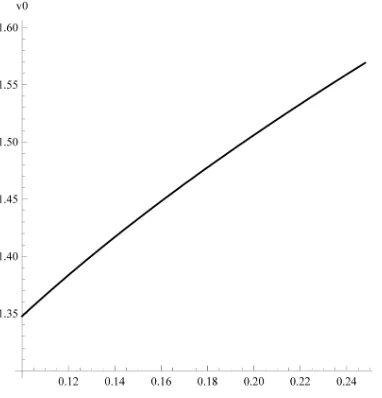
set r0.1, 0.09, 0.3, 1, 0,d p q
150, 3 . Using these parameters,
is 0.248.
[image:7.595.217.408.525.724.2]
Figure 1 shows how the optimal exercise boundary increase as the penalty increases from 0.1 up to . From the figure, we can see that the optimal boundary v0 is increasing in the penalty . Figure 2 demons
Figure 2. The value function.
tes the value function of Game Russian option with jumps. Dashed lines represent the graph of the value V in 0.1, 0.15
from the bottom, respectively. Real line represents the value in 0.2. From Figure 2, can nize that is convex and increasing in
5. Conclusion
In this paper, we discussed the valuation of Game Russian option written on dividend paying asset, obtained the value function of it for double exponential jump diffusion processes and also explored some analytical proper- ties of the value function and the optimal boundaries for the seller and buyer, which were useful to provide an approximation of the finite lived Game Russian option. Moreover, we plan to examine convertible bonds with jumps by using Game option frame work. We shall leave it as future work.
REFERENCES
[1] Shepp, L.A. and Shiryaev, A.N. (1993) The Russian option: Reduced regret. The Annals of Applied Probability, 3, 631-640. http://dx.doi.org/10.1214/aoap/1177005355
we
visually recog V
v v.[2] Shepp, L.A. and Shiryaev, A.N. (1994) A new lo tion”. Theory of Probability and Its Applica- tions , 103-119. http://dx.doi.org/10.1137/1139
ok at pricing of the “Russian op 004
, 39
[3] Kifer, Y. (2000) Game options. Finance and Stochastics, 4, 443-463. http://dx.doi.org/10.1007/PL00013527
Karatzas, I. (1996) Backward stochastic differential equations with reflecti ynkin games. The Annals of robability, 24, 2024-2056.
[4] Cvitanic, J. and on and D
P http://dx.doi.org/10.1214/aop/1041903216
[5] Kyprianou, A.E. (2004) Some calculations for Israeli options. Finance and Stochastics, 8, 73-86. g/10.1007/s00780-003-0104-5
http://dx.doi.or [6] Su
M
zuki, A. and Sawaki, K. (2009) The pricing of callable Russian options and their optimal boundaries. Journal of Applied athematics and Decision Sciences, 2009, Article ID: 593986, 13 p. http://dx.doi.org/10.1155/2009/593986
ou, S.G. and Wang, H. (2004) Option pricing under a double exponential jump diffusion model. Management Science, 50, 78-1192.
[7] K
11 http://dx.doi.org/10.1287/mnsc.1030.0163
zuki, A. and Sawaki, K. (2010) The valuation of Russian options for double exponential jump diffusion processes. Asia Pa- fic Journal of Operational Research, 27, 227-242.
[8] Su ci
[9] Kou, S.G. and Wang, H. (2003) First passage time ss. Advances in Applied Probability, 35, 504-531. http://dx.doi.org/10.1239/aap/1051201658
s for a jump diffusion proce
-[10] Sato, K. and Suzuki, A. (2011) Stochastic cash management problem with double exponential jump diffusion processes. Lec