Published Online January 2014 (http://www.scirp.org/journal/ojbm) http://dx.doi.org/10.4236/ojbm.2014.21009
Management Analysis of Industrial Production Losses by
the Design of Experiments, Statistical Process Control, and
Capability Indices
Djida Bounazef
1,2, Smain Chabani
1, Abdelhafid Idir
1, Mokhtar Bounazef
31
HEC, Commercial Graduate School of Algiers, Algiers, Algeria
2Abderrahmane Mira University of Bejaia, Bejaia, Algeria 3
Djillali Liabes University of Sidi Bel Abbes, Sidi Bel Abbes, Algeria
Email: [email protected], [email protected], [email protected], [email protected]
Received November 21, 2013; revised December 23, 2013; accepted January 10, 2014
Copyright © 2014 Djida Bounazef et al. This is an open access article distributed under the Creative Commons Attribution License, which permits unrestricted use, distribution, and reproduction in any medium, provided the original work is properly cited. In accor-dance of the Creative Commons Attribution License all Copyrights © 2014 are reserved for SCIRP and the owner of the intellectual property Djida Bounazef et al. All Copyright © 2014 are guarded by law and by SCIRP as a guardian.
ABSTRACT
The machine stops caused by various breakdowns, rupture of raw materials, production changes, scheduled maintenance and stops related to human resources management generate an important production loss in the company. Our case study is done in a company that manufactures polyethylene pipes with eight production lines. They stop frequently because they undergo external control factors and noise factors. The method of experi- mental design that relies on statistical surveys is applied to production loss allows us to observe the action of each factor on the loss of production and their interactions of these factors combined in pairs on this process. Analysis of results shows the dominance of controllable or uncontrollable factor on the loss of production. This is illus- trated by response surfaces and ISO responses lines were derived by mathematical modelling. Solutions are proposed to improve continuous production, reduce waste and scrap and therefore increase profitability of company.
KEYWORDS
Design of Experiments; Production Losses; Response Surfaces; Polynomial Modelling; Integrated Management System
1. Introduction
The reduction of industrial waste is the major preoccupa-tion of an integrated management system [1,2] which includes the environmental management system [3], the system of quality management [4,5] and the management system of health, security and work [6,7]. These sys-
tems are applied within the company following the re-
quirements of ISO 9001:2000 code 4, until 8.5.3, of ISO 14001:2004 and OHSAS 18001:2007 to achieve optimal production by minimising work stops caused by various technical and operational reasons. This integrated mana- gement system [8-10] is applied to the production lines at the beginning when checking the quality of raw materials until the end when storing finished products to contribute in reducing production losses and obtaining finished
quality products. For this, the checks are carried out to the quality of raw materials, during the production proc-
ess, for finished products and after handling and storage. However, the implementation of integrated management system is not sufficient in itself, in parallel it is necessary to reduce production stops caused by mechanical and electrical problems, by human resources management, by the supplies disruption of raw materials and others. To know the influence of each breakdown reason of ma-
chinery at each production line, a data record has been established for a period of one year. These causes were grouped into 3 categories that encompass these machine stops into the same types. These categories are the acci-
2. Statistical Reports of the Causes of
Production Stops
Modelling by design of experiments method analyses the continuous production process of polyethylene pipes by measuring causes of production losses (waste) caused by the steering factors and noise factors. The causes of ma- chines downtimes that increase the percentage of produc- tion loses (inducing the waste) are defined by three pa- rameters on the Ishikawa diagram (Figure 1).
The production process is composed of eight inde- pendent production lines; their stops are caused sepa- rately by the same reasons and therefore act on produc- tion losses (lack of production).
Table 1 shows the distribution of hours of production losses by types and production lines. The accidental stops are designed by X1, the scheduled stops are designed by
X2 and the stops due to raw material and finished prod-
ucts are designed by X3. Table 1 is called matrix of ex-
periments, it contains column 6 that means losses of production expressed in percent. They designate the re- sponses Y. We see that the line E records the high num- bers of hours of accidental stops with 2731.83 hours and human resources management stops with 1085.67 hours, but it is the line H that has the high number of Stopsdue to raw material and finished products with 9703.75 hours. The greatest loss of production is recorded on line E with 66.18% compared to optimal production. This is the line that stores the most breakdowns and stops. However, it is the line C that has the smallest losses of production with 20%.
3. Phenomenon Analysis of Machines Stops
by Design of Experiments Method
The loss of industrial production caused mainly by dif-ferent stops responds to a mathematical law in polyno-mial form. This polynopolyno-mial is a sum of monopolyno-mials that are composed of coefficient ai (called parameter effect)
multiplied by the value of the parameter designated by xi.
In our study, x1 is letter that represents accidental stops,
x2 isletter that represents maintenance and human re-
sources management stops, and x3 represents stops due to
raw material and finished products. In the polynomial, there are monomials that designate the interactions be- tween the parameters that influence the result; these pa-
values. Generally they are coded because their units and their scales that affect the response “y” are different. For each parameter, we denote by (−1) the minimum value, and by (+1) the maximum value; the intermediate values are calculated by the following formula:
min max
max min
2
2 i
i
u u
u x
u u
+
−
=
−
(2)
where: Umin is minimal value of parameter, Umax: is
maximal value of parameter, Ui is value to be encoded,
and xi is coded value.Table 2 shows these coded values.
The matrices calculation allows us to obtain the effects values aiof parameters by forming 10 different equations
from equation 1 by replacing the xi parameters by values
from Table 1, we could obtain the 10 coefficients ai,j by
the following formula:
(
)
1t t
a= X X − X Y (3) Substituting the values of ai,j into Equation (1), the
production losses caused by three types of stops is mod-elled by the following expression:
1 2 3
1 2 1 3 2 3
2 2 2
1 2 3
37.8259 6.81969 1.90399 2.03238 1.30382 8.78769 2.8691 1.42286 2.72951 0.44013
y x x x
x x x x x x
x x x
= + + +
+ − −
− + +
(4)
4. Results Interpretation
The interpretation is subdivided in two essential parts, the first consists to analyse causes of production stops of 8 lines of production using design of experiments method, while the second consists to analyse waste generated by frequency of production stops using statistical process control.
5. Analysis of Production Stops Effects by
Experiments Design Method
Equation (4) allows us not only to find the real loss val-ues of production “y” listed in Table 2, but other values included between the maximum and minimum losses. This is a predictive and descriptive model. This is shown by the estimators of adjusted descriptive quality Radjust2
67
[image:3.595.58.539.231.367.2]Figure 1. Stops due to raw material and finished products.
Table 1. Hours of production losses per line.
N˚ Lines Accidental stops [H] (X1)
Maintenance and human resources management stops
[H] (X2)
Stops due to raw material and finished products
[H] (X3)
Production losses [%] (Y)
1 Line A 220.8 798.92 988.08 22.49
2 Line B 1692.8 844.08 1048 40
3 Line C 153.67 815.75 795.08 20
4 Line D 1891.75 669.42 1291.83 43.27
5 Line E 2731.83 1085.67 2074.75 66.18
6 Line F 1393.5 876.92 1515.58 42.52
7 Line G 741.88 859.67 779.17 26.74
8 Line H 1690.33 795.61 9703.75 41.26
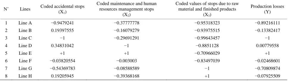
Table 2. Coded values of several stops of machines.
N˚ Lines Coded accidental stops (X1)
Coded maintenance and human resources management stops
(X2)
Coded values of stops due to raw material and finished products
(X3)
Production losses (Y)
1 Line A −0.9479241 −0.37777778 −0.95318323 −0.89216111 2 Line B 0.19397555 −0.16079279 −0.93975515 −0.13382417
3 Line C −1 −0.29691291 −0.99643457 −1
4 Line D 0.34831042 −1 −0.8851128 0.00779558
5 Line E +1 +1 −0.70966029 +1
6 Line F −0.03820554 −0.003003 −0.83497039 −0.02468601
7 Line G −0.54369783 −0.08588589 −1 −0.70809874
8 Line H 0.19205945 −0.39368168 +1 −0.07925509
values are numbers usually between ‒∞ and 1. Values close to 1 for both Radjust2 and Q2 indicate very good model with excellent predictive result. In our case
2
adjust 0.903
R = and Q2 = 0.863. The first estimator re-flects the contribution of the model in the restitution of the observed response and the second estimated coeffi-cient reflects the ability of the model to predict response without making statistical measurements or experiments. To illustrate these results, the Figure 2 shows the devia-tions of measurement points relative to bisector.
The details of deviations are shown in Table 3 where one sees that the maximum deviation is estimated to 7.9% in measurement 7. The Student test shows us if the vari-able xi or the interaction xi,jassociated with ai,j affects
response “y” or not. For this, one calculates the coeffi-cient ti of Student as follows:
i i
i
a t
s
= (5)
With 2
i
s is variance of effects; it is calculated by fol-lowing:
2 2
i s s
n
= (6)
where s2 is estimator of polynomial effects; it is calcu-lates by this formula:
2 1 2
i
s e
n p =
−
∑
(7)Here, n is equations number obtained by combinations of values of xi,j from Table 1, it is equal to 3
3
[image:3.595.56.540.398.539.2]20 30 40 50 60 Predicted
[image:4.595.306.539.252.508.2]Figure 2. Observed vs. Predicted plot.
Table 3. Deviations between predicted and observed values.
N˚ Observed Predicted Difference
1 22.49 21.6865 0.803453
2 40 41.2669 −1.26685
3 20 19.7343 0.265732
4 43.27 43.4725 −0.202545
5 66.18 66.331 −0.151001
6 42.52 39.1532 3.36685
7 26.74 29.5363 −2.79629
8 41.26 41.2793 −0.0193405
cients, it is equal to 10 (see Equation (1)). The compari-son between tcrit taken from Student table for risk α =
0.05 and freedom degree ν = 17, shows that all “ti” are
higher than tcrit = 0.689, it means that all variables xi,j
influence the response “y”, i.e. the loss of production (Table 4).
Equation (4) allows working simultaneously the three parameters in the field of work but we cannot interpret it graphically. However, we vary two parameters while leaving unchanged the third parameter (x3).
6. Production Losses
According Accidental
Stops When x
2and x
3Are Middle Values
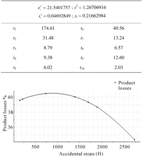
To observe how the losses of production vary according one parameter, one gives to 2 others parameters in Equa-tion (4) permanent middle values. We can thenplot the variation of production losses according one of 3 pa-rameters. The statistics collected during the production indicate that while stabilising the production losses due to raw materials and finished products as well as main-tenance to their middle values (x2 = 877.7 hours, x3 =
5241.6 hours), one reaches the maximum value of 40.5% of production losses at 900 hours of accidental stops. The mathematical modelling decreases these losses to 34.3% at 2730 hours (Figure 3). When x1 exceeds the value of
900 hours, x2 and x3 are statistically acting on the model
and are decreasing production losses.
Table 4. Student coefficients.
2
21.5401757
i
e = ; s2 = 1.26706916 2
0.04692849
i
s = ; si= 0.21662984
t1 174.61 t6 40.56
t2 31.48 t7 13.24
t3 8.79 t8 6.57
t4 9.38 t9 12.60
t5 6.02 t10 2.03
Figure 3. Graph of production losses according accidental stops.
7. Production Losses
According
Maintenance and Human Resources
Management Stops When x
1and x
3Are
Middle Values
Maintaining accidental stops x1 and stops due to raw
ma-terial and finished products x3 constant respectively at
1476.40 hours and 5241.6 hours, one varies only x2 from
its minimum value to its maximum value, we obtain a minimal loss of production of 39.8% for x2 = 860 hours
(Figure 4).
This means that the parameter x2 has a positive
influ-ence in reducing production losses in the model (4), but from x2 = 860 hours, factors x1 and x3 are more influential
than x2. This explains why the curve increases until
[image:4.595.57.288.253.393.2]69
Figure 4. Graph of production losses according mainte-nance and human resources management stops.
8. Production Losses
According Stops Due to
Raw Material and Finished Products
When x
1and x
2Are Middle Values
When we leave constant x1 = 1476.40 hours and x2 =
877.70 hours (middle values), we note that the minimum losses of production is quickly reached at 30.8% for x3 =
3260 hours when the curve decreases. This shows that from this minimum, the factors x1 and x2 are increasing
the response “y” (production losses) when x3 varies from
its minimum value to maximum value (Figure 5).
9. Results Interpretation When x
1and x
2Are Varied Together
For this, one gives to third parameter x3 an invariable
value and one changes the 2 other from their minimum value to their maximum value. One can plot response surfaces in three dimensions and curves iso-responses in two dimensions to illustrate the action of two parameters simultaneously on the production losses.
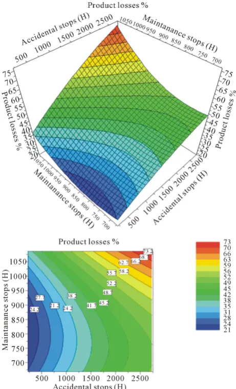
10. When x
3Is Equal at the Low Value
(x
3= 779.17 Hours)
In this case, the response surface is concave rectangular form; it shows parallel areas of production losses mainly when accidental stops (x1) and stops caused by
mainte-nance and management of human resources (x2) are high
(Figure 6).
When accidental stops are less than 1500 hours, these areas are parallel to the axis of x2. It shows that
acciden-tal stops act very low in the model response. All this is visible on curves ISO response, where one notes that the losses of production remains relatively constant between 20.8% and 24.2% for stops due to maintenance and management of human resources between 675 hours and 937.5 hours. From 1330 hours of accidental stops that the increase of x2 increases clearly the production losses.
11. When x
3Is Equal at the Middle Value
(x
3= 5241.60 Hours)
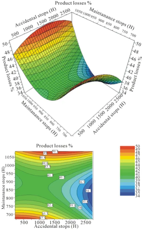
[image:5.595.59.289.94.196.2]When x3 takes the middle value of 5241.6 hours, the ma-
Figure 5. Graph of production losses according stops due raw material and finished products.
Figure 6. Response surface and ISO response curves when x3 is low.
thematical model (4) presents responses surface as a sad-dle of horse (Figure 7). Its complexity shows how the simultaneous influence of x1 and x2 acts on production
[image:5.595.307.538.243.623.2]Figure 7. Response surface and ISO response curves when x3 is middle.
tacles.In this section, the response “y” remains relatively constant; it varies from 40.5% to 41.3% over a large part of the work domain.This shows that we can get the con-stant value of production losses defined by the 41.3% by several combinations between accidental stops (x1) and
maintenance and management of human resources stops.
Table 5 gives some values of production losses outside the central zone with tentacles.
It is clear, that the columns and rows (Table 5) display for constant values of the parameter x1, that production
losses decrease in first with increasing parameter x2,
sta-bilise at central area of the graph 8, and subsequently increase.However, when x2 remains constant, production
losses decrease for the 2 first rows with increasing x1, but
increase in first and subsequently decrease for the 2 last rows ofTable 5 with increasing x1.
12. When x
3Is Equal at the High Value
(x
3= 9703.75 Hours)
When the parameter x3 takes its maximum and invariable
hours 42.7% 43.8% 43.9% 43.1% 41.4% 1050
hours 45.5% 46.9% 47.3% 46.8% 45.4%
value of 9703.75 hours in the mathematical model 4, the responses surface is the concave form upwards (Figure 8). Its projection gives curves ISO responses directed from top to bottom and curved in the centre of the graph.This shows that for a given value of accidental stops (x1),
losses of production vary slowly with the change of stops due to maintenance and human resource management. It is easy to see that for maximum value of x3 = 9703.75
hours, the increase of accidental stops (x1) reduced the
losses of production; this is due to the effect of negative sign of the interaction of parameters x1 and x3 in the
polynomial (4) and equal to a13 = −8.78769 which
re-duces considerably the value of the response “y”. One remarks that in passing from value x1 = 500 hours to
x1=2500 hours for the same value of x2 = 900 hours,
losses of production fells from 55.8% to 22.2%.
13. Management of Production Waste by
Statistical Process Control
The losses rate of production per lines caused by the various stops does not explain alone the waste of finished products during production process. It is rather frequency of repeated stops that causes restarts manufacturing process. This will requires each time the equipments set-tings to obtain the finished standardised products. Know- ing annual waste rate of polyethylene products for water of 3.15% and for gas of 2.54%, the average waste rate of 8 lines is:
1
Waste rate 2.845%
n i i
x n
=
=
∑
= (8)where:
∑
xi is sum of distribution values equal to 5.69%; n is samples number equal to 2; this is giving us process quality “m” or “Yield” of 97.155% (Figure 9).This value is considered as the average value of the process target to achieve (average value of distribution). As the value of the standard deviation is sigma equal to 0.9425071, the repetition frequency of production stops is:
1
0.42328 2π
f σ
[image:6.595.310.537.102.220.2]71
Figure 8. Response surface and ISO response curves when x3 is high.
This value is represented by the top of the Gauss curve of production process. It corresponds to 0.91569σ on the X axis and represents the lag due to the production proc-ess and waste estimated at 28500 DPMO (defects per millions of opportunities) (Unhatched area of Figure 9). The beginning of waste area corresponding to end of process performance z, it is found in the following man-ner:
coef
z= ⋅σ (10) where z is sigma process quality; it is calculated with coefficient who taken from the normal distribution taking account the risk of 0.05 and “UCL, LCL” values through manufactured tables (coef = 3.403311); the process per-formance z is equal at 3.403311σ. The σ value is the standard deviation, it calculated by this formula:
(
)
2 1n i
x m
n σ
−
[image:7.595.56.285.87.464.2]=
∑
(11)Figure 9. Gauss curve of production losses.
The process performance z is then 3.2076447. The low control limit (LCL) and the upper control limit (UCL) are calculated by this following formula; here, the target is the process quality m = 100% ‒ 2.845% = 97.155%:
LCL, UCL=target±3σ (12) Their respective values are then 94.327419 and 100.377521. The process quality area of the real produc-tion process is thus defined by LCL, UCL and the Gauss curve of normal distribution (hatched zone in Figure 9). It is equal to 97.155%. The combination of two methods of analysis, the experimental design and statistical proc-ess control in management showed us that performance of studied process is relatively small compared to a process without stops or waste. The management of waste during the production process is directly linked to the frequency of stops and starts of manufacturing lines. To achieve Six Sigma process with performance of 99.999%, one must improve the process capability index
Cpin order to be higher than 2. However, the capability
index of six production lines is z/3 = 1.1344; the produc-tion process of PE is then just capable. To achieve high performance, one must act in several fields that cause the increase of waste. Managing production waste is to un-derstand the real causes that push businessmen to submit program changes on the production lines, and see if there are opportunities for their reductions. It must also under-stand the real causes of mechanical and electrical failures and assess the reliability of the maintenance planning. Finally know the real causes of non conformities of products and analyse the production process and inter-vention function responsible for the technical quality. Thereafter take the necessary technical and financial measures and control by means of managerial actions to reduce this waste.
14. Capability Indices and Process
Performance
The capability indices of process “Cp”, of machine “Cm”
and process performance “Pp” are important data that de-
following manner:
3.2076447
1.0692149
3 3
p z
C = = = (14)
The Cp index exceeds the value of 1, but the quality of
process 6σ requires a capability of process more than 2. The production process of the tubes is barely capable but is not very efficient. The capability index of Machine Cm
allows measuring the material resources available the continuous production process of the tubes is able to achieve the target of 99.999966% of performance; the value of this index is:
(
)
2 1UCL LCL ; 3
target ; 1 0.6292
m
n i i
m
C
x n C
σ
σ =
− =
− =
− =
∑
(15)
The Cm index does not exceed 1.11 which allows the
reduction of waste of 0.00034%. The tools and machin-eries of production plant are not capable to achieve per-formance of 6σ quality. The plant must innovate and re-duce the variability due to different causes of machine stops.
15. Conclusion
Causes analysis of waste by 2 methods statistical process control and design of experiments are a very effective means that can take measures to manage the losses. These methods permit to develop recommendations. They can satisfy demands to achieve the production re-quirements mastering the controllable factors, reducing the impact of uncontrollable factors, minimising the fi-nancial losses and improving the quality of production. The reduction of waste is the result of the reduction of machine stops; this reduction supports the achievement
Equation (10).
REFERENCES
[1] P. Bousselet, “The process Computerisation QSE in Ag- ribusiness: The 30 Questions to Consider Quality, Safety and Environment,” PBC Soft, Paris, 2010.
[2] B. Froman, J. M. Gey and F. Bonnifet, “Quality, Safety and Environment: Construct an Integrated Management System,” AFNOR, La Plaine Saint-Denis, 2007.
[3] M. Bernardo, M. Casadesus and S. Karapetrovic, “How Integrated Are Environmental, Quality and Other Stan-dardised Management Systems? An Empirical Study,” Journal of Cleaner Production, Vol. 17, No. 8, 2009, pp. 742-750.http://dx.doi.org/10.1016/j.jclepro.2008.11.003 [4] K. R. Bhote, “The Power of Ultimate Six Sigma, Quality
Excellence to Total Business Excellence,” Amacom, New York, 2003.
[5] D. Duret and M. Pillet, “Quality in Production: From ISO 9000 to Six Sigma,” 4th Edition, Eyrolles Edition, Paris, 2005.
[6] H. Aadi and B. John, “Hygiene and Safety at Work,” Office of Professional Training and Work Promotion, Rabat, 2011.
[7] Fernandez-Toro and A. H. Schauer, “Management of Information Security: Implementing ISO 27001, Imple-mentation of ISMS and Certification Audit,” Eyrolles, Paris, 2008.
[8] R. Holdsworth, “Practical Applications Approach to De- sign, Development and Implementation of an Integrated Management System,” Journal of Hazardous Materials, Vol. 104, No. 1-3, 2003, pp. 193-205.
http://dx.doi.org/10.1016/j.jhazmat.2003.08.001
[9] T. H. Jorgensen, A. Remmen and M. D. Mellado, “Inte-grated Management Systems—Three Levels of Integra-tion,” Journal of Cleaner Production, Vol. 14, 2006, pp. 713-722.