CMS swaps in separable one factor Gaussian LLM and HJM model

Munich Personal RePEc Archive

CMS swaps in separable one-factor

Gaussian LLM and HJM model

Henrard, Marc

Bank for International Settlements

8 May 2007

MODEL

MARC HENRARD

Abstract. An approximation approach to Constant Maturity Swaps (CMS) pricing in the sep-arable one-factor Gaussian LLM and HJM models is presented. The approximation used is a Taylor expansion on the swap rate as a function of a random variable which is intuitively similar to a (short) rate. This approach is different from the standard approach in CMS where the discounting is written as a function of the swap rate. The approximation is very efficient. Copyright c2006–2007 by Marc Henrard.

1. Introduction

Constant Maturity Swaps (CMS) are easy to describe and at first sight may seem easy to price. A CMS is composed of several payments. Like for the floating leg of a standard IRS the payment are done on a regular short term basis (typically three or six months). The rate fixing take place two1_{business days before the start of the period. The rate is multiplied by the accrual factor of} the period and paid at the end. The difference with the floating leg of an IRS is that the rate used for the fixing is not the rate corresponding to the period but a swap rate. The tenor of the swap is longer than the one of the payment period; typically the tenor is five or ten year.

The valuation involved both the swap rate and the discounting from the payment date. The price is usually obtained using some approximations. The standard approach is to approximate the discounting to payment date adjusted by the numeraire by a function of the swap rate. Then further approximation (often of order two) is required to obtain an explicit price. This approach is briefly described inHull(2006) and in a more general and detailed way inHagan(2003).

In this paper the CMS are studied in two different models: the one-factor separable Gaussian LMM and HJM models. For the HJM model, the term Gaussian refers to a model where the volatility is deterministic and the instantaneous forward rate are normally distributed. For the LMM, the term Gaussian refers to the model where the Libor rates satisfy a Bachelier-type equation

dLt=σdWtand the rates are normally distributed (in their own forward measure). The models are discribed with more details in the next section.

A different approach to the standard one is used for the approximation. The exact swap rate and the discounting are written as function of an underlying random variable. Intuitively the variable is the stochastic integral of the volatility along the underlying Brownian motion. In the models used the rates are normally distributed and the rates are more or less linear in the variable. The “more or less” comes from the fact that in both models it is not the swap rate which is modelled and normally distributed but respectively the instantaneous forward and the Libor rates. Nevertheless using a Taylor expansion of the swap rate in term of the underlying random variable, very precise results can be obtained. Moreover by expanding around a specific point (which is not 0), the symmetry of the distribution can be used to obtain a price expansion with only even terms; one order of approximation is obtained for free.

Date: First version: 7 July 2006; this version: 8 May 2007.

Key words and phrases. CMS swap, LLM model, HJM model, one factor, approximation. JEL classification: G13, E43, C63.

AMS mathematics subject classification: 91B28, 91B24, 91B70, 60G15, 65C05, 65C30.

1_{The fixing lag is two business days in most of the currencies, the GBP being the most noticeable exception.}

2 M. HENRARD

The CMS prices are often described in term ofadjusted forward rate (including in some places in this note). There is no reason why the forward rate should be used in the computation except a similarity with a standard swap where the floating payment can be valued using the forward rate discounted to today. Also it is usually easier to express the valuation in term of rate than in term of price. The price of a CMS payment can be written as the discounted expected value of the forward rate multiplied by a factor. The adjustement is not only in the factor but also in the fact that the expected value is not taken in the measure for which the rate is a martingale.

2. Model and hypothesis

In general, the HJM framework describes the behavior of P(t, u), the price in t of the zero-coupon bond paying 1 inu(0≤t, u≤T). When the discount curveP(t, .) is absolutely continuous, which is something that is always the case in practice as the curve is constructed by some kind of interpolation, there existsf(t, u) such that

(1) P(t, u) = exp

−

Z u

t

f(t, s)ds

.

The idea of Heath et al. (1992) was to exploit this property by modeling f with a stochastic differential equation

df(t, u) =µ(t, u)dt+σ(t, u).dWt

for some suitable (potentially stochastic)µandσand deducing the behavior ofP from there. To ensure the arbitrage-free property of the model, a relationship between the drift and the volatility is required. The model technical details can be found in the original paper or in the chapter

Dynamical term structure model ofHunt and Kennedy(2004).

The probability space is (Ω,{Ft},F,P). The filtration Ft is the (augmented) filtration of a

one-dimensional standard Brownian motion (Wt)0≤t≤T. To simplify the writing in the rest of the

paper, the notation

ν(t, u) =

Z u

t

σ(t, s)ds

is used.

Let Nt = exp(Rt

0rsds) be the cash-account numeraire with (rs)0≤s≤T the short rate given by

rt=f(t, t). The equations of the model in the numeraire measure associated toNtare

df(t, u) =σ(t, u)ν(t, u)dt+σ(t, u)dWt

or

dPN(t, u) =−PN(t, u)ν(t, u)dWt

The notationPN_{(t, s) designates the numeraire rebased value of P, i.e.P}N_{(t, s) =N}−1

t P(t, s).

The following technical lemma was presented in Henrard (2005) for the Gaussian one-factor HJM. Similar formulas can be found in (Brody and Hughston,2004, (3.3),(3.4)) in the framework of coherent interest-rate models.

Lemma 1. _{Let 0≤θ≤t0≤ti. In the HJM framework the price of the zero coupon bond is}

P(θ, ti) =P(0, ti)

P(0, θ)exp −

Z θ

0

(ν(s, ti)−ν(s, θ))dWs−1

2

Z θ

0

ν2_{(s, ti)−ν}2_{(s, θ)}

ds

!

.

To be able to use the explicit formula for the valuation of the European swaptions, we will also use the following hypothesis.

H1: _{The functionσsatisfiesσ(t, u) =g(t)h(u) for some positive functiongandh.}

The idea behind the Libor Market model is to embed different Black-like equations for the forward (Libor) rate between standard dates (0≤t0 < t1<· · ·< tn) into a unique HJM model. The Libor ratesL(t, tj) are defined by

1 +δiL(s, ti) = P(s, ti)

The equations underlying the Bachelier (or normal or Gaussian) Libor Market Model are

(2) dL(t, tj) =γj(L(t, tj), t)dWtj+1

in the probability space with numeraire P(t, tj+1). Theγj (0 ≤j ≤n−1) are one-dimensional functions. To merit the full qualification of Bachelier model, γj should be purely deterministic (not involving L). For fundamental reasons explained in the appendix of Henrard (2007) such a model would be ill-defined. In this section the γ are used with their most general form. The next section will consider them in their simple deterministic form (with the understanding that they are modified far away from reasonable rates as suggested in Henrard(2007) to obtain a well defined model). The coefficients can be considered also as affine functions leading to a displaced log-normal dynamic as also described in appendix of the above mentioned paper.

The Brownian motion change between theNtand theP(t, tj+1) numeraires is given by

dWtj+1=dWt+ν(t, tj+1)dt.

The differenceν(t, tj+1)−ν(t, tj) can be written as

ν(t, tj+1)−ν(t, tj) = 1

L(t, tj) + 1

δj

γj(L(t, tj), t)

The model will be studied under the separability conditions

H2: _{γj(s) =βjγ(s) withβj>0 andγ(s)>0.}

As mentionned in the introduction, this type of conditions appeared in interest rate modelling in different circumstances. The reader is reffered toPelsser et al.(2004) for more on thisnonrestrictive requirement in the LLM framework.

3. CMS pricing

The price of the CMS payments are analysed in the two models described in the previous section. The fixing of the swap rate take place in θ for a swap with reference dates{ti}0≤i≤n. The first

date t0 is the settlement date, the next are the coupon payments, and the maturity is intn. The accrual fraction of the different periods of the swap are {γi}1≤i≤n. The rate obtained is paid in tp≥θ with an accrual fractionφusually corresponding with the periodt0−tp.

The numeraire is changed to the priceP(t, θ). The associated Brownian motion isWθ

t given by dWθ

t =dWt+ν(t, θ)dt. With that change of numeraire and Lemma1, the price of the zero-coupon

is

P(θ, ti) = P(0, ti)

P(0, θ) exp −

Z θ

0

ν(s, ti)−ν(s, θ)dWsθ−

1 2

Z θ

0

(ν(s, ti)−ν(s, θ))2ds

!

.

In the Guassian HJM, the volatility is deterministic and the integrals can be written explicitely. Let

(3) (αiG)

2 =

Z θ

0

(ν(s, ti)−ν(s, θ))2ds.

The price of the zero-coupon is then

P(θ, ti) =P(0, ti)

P(0, θ)exp

−αGi X− −

1 2(α

G i )2

with X standard normally distributed. Like inHenrard (2003) and Henrard(2006) the random valiable X is the same for all the maturities thanks to the separability hypothesis (H1).

In the normal LMM, the volatility is not deterministic any more and approximations are used:

ν(s, ti)−ν(s, θ)≃ν(s, ti)−ν(s, t0).

4 M. HENRARD

The difference can be written in term of the LMM parameters

ν(s, ti)−ν(s, θ) ≃

i−1 X

j=0

ν(s, tj+1)−ν(s, tj) (4)

=

i−1 X

j=0

γj(s)

Li s+ 1/δj

.

(5)

The last term contains the random variablesLi

s. Like inHenrard(2007) the value on the path can

be approximated by its initial value Lj0. Using the notations

λj = 1

Lj0+ 1/δj

, Γ2₌

Z θ

0

γ2_(s)ds,

(6) αLi =

i−1 X

j=0

λjβjΓ

one obtains

ν(s, ti)−ν(s, θ)≃

i−1 X

j=0

λjβjγ(s).

The two integrals appearing in the zero-coupon bond price become

Z θ

0

ν(s, ti)−ν(s, θ)dWsθ≃αLiX and

Z θ

0

(ν(s, ti)−ν(s, θ))2_ds≃(αL i)2.

For both models, the price of the zero-coupon is approximated by

P(θ, ti)≃ P(0, ti)

P(0, θ) exp

−αiLX−

1 2(α

L i)

2

.

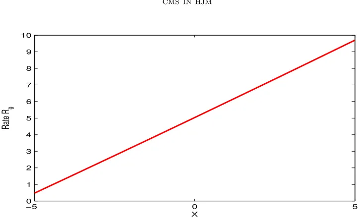
The swap rate is

Rθ(X)≃P(0, s0) exp −α0X−

1 2α

2 0

−P(0, sn) exp −αnX−1 2α

2

n

Pn

i=1γiP(0, si) exp −αiX− 1 2α

2

i

The rate is almost linear in the variableX. The graph ofRθ forX between -5 and 5 is given in Figure1.

For the two models the zero-coupon price can be written in the same way. The difference is that one is exact and the other is an approximation. Also the meaning of the constantsαi are different.

Theorem 1. _{In the separable one-factor Gaussian HJM and normal LMM the price of the CMS}

payment is approximated to the order mby

V0m=φP(0, tp) 

A0+

⌊m/2⌋

X

i=1

A2i

2i_i!





where⌊r⌋is the integer part ofr and the coefficientAi are the one of the Taylor expansion of Rθ

aroundαp:

Rθ(X) =

m

X

i=0 1

i!Ai(X+αp)

i

and the coefficientsαare given respectively by (3) and (6).

Proof. The CMS pays the swap rateRθ fixed inθat the payment datetp. The value of one CMS payment at the fixing date is φRθP(θ, tp). Using the P(t, θ) numeraire the value is

V0 = φP(0, θ) E [RθP(θ, tp)] (7)

= φP(0, tp) E

Rθ(X) exp(−αpX−α2

p/2)

.

−5 0 5 0

1 2 3 4 5 6 7 8 9 10

X

Rate R

θ

Figure 1. Swap rateRθ as function of the underlying random variableX.

Using the expansion ofRθ(X) around−αpone only needs to compute the expected values

E

(X+αp)iexp

−αpX−1

2α 2

p

=

 



0 iodd

1 i= 0

Qi/2

j=1(2j−1) ieven The result is obtained by notting that the product can be written as a factorial:

i

Y

j=1

(2j−1) = (2i−1)! 2i−1_(i−1)!.

Note that only the even terms appear in the final price. An approximation of order 3 can be obtained withA0 andA2 only. By addingA4, one has an approximation of order 5. To the order 4, the price is

φP(0, tp)(A0+A2/2 +A4/8).

The explicit computation of the factorsAicorresponding to the Taylor expansion ofRθ aroundαp

is quite long. In our implementation the factorsAo andA2 are computed explicitely. The formula forA2(second order derivative) take around ten lines of code. The factorA4 is computed through a numerical computation as teh second order derivative ofA2:

A4= (A2(αp+ǫ) +A2(αp−ǫ)−2A2(αp))/ǫ2.

The next section shows that in practice it is enough to use the second order development.

4. Implementation

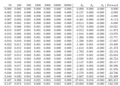
The approximation with terms up toA0,A2andA4are compared with a numerical integration approach to assess the precision of the approximation for the Hull-White extended Vasicek model. The example is a 10y x 10y semi-annual CMS with a flat curve at 5% and Vasicek parameters (a, σ) = (0.01,0.01).

6 M. HENRARD

50 100 500 1000 5000 10000 50000 A0 A2 A4 Forward 0.000 0.000 0.000 0.000 0.000 0.000 0.000 0.000 0.000 0.000 0.000 0.002 0.001 0.000 0.000 0.000 0.000 0.000 -0.157 0.000 -0.000 -2.093 0.005 0.002 0.000 0.000 0.000 0.000 0.000 -0.312 0.000 -0.000 -4.080 0.007 0.003 0.001 0.000 0.000 0.000 0.000 -0.461 0.000 -0.000 -6.113 0.009 0.005 0.001 0.000 0.000 0.000 0.000 -0.614 0.000 -0.000 -8.080 0.011 0.006 0.001 0.001 0.000 0.000 0.000 -0.753 0.000 -0.000 -10.021 0.013 0.007 0.001 0.001 0.000 0.000 0.000 -0.912 0.000 -0.000 -11.972 0.016 0.008 0.002 0.001 0.000 0.000 0.000 -1.044 0.000 -0.000 -13.870 0.018 0.009 0.002 0.001 0.000 0.000 0.000 -1.200 0.000 -0.000 -15.771 0.019 0.010 0.002 0.001 0.000 0.000 0.000 -1.330 0.001 -0.000 -17.687 0.022 0.011 0.002 0.001 0.000 0.000 0.000 -1.488 0.001 -0.000 -19.498 0.023 0.012 0.002 0.001 0.000 0.000 0.000 -1.612 0.001 -0.000 -21.373 0.026 0.013 0.003 0.001 0.000 0.000 0.000 -1.763 0.001 -0.000 -23.134 0.027 0.014 0.003 0.001 0.000 0.000 0.000 -1.878 0.001 -0.000 -25.034 0.030 0.015 0.003 0.002 0.000 0.000 0.000 -2.038 0.001 -0.000 -26.724 0.032 0.016 0.003 0.002 0.000 0.000 0.000 -2.147 0.001 -0.000 -28.517 0.033 0.017 0.003 0.002 0.000 0.000 0.000 -2.303 0.002 -0.000 -30.296 0.036 0.018 0.004 0.002 0.000 0.000 0.000 -2.405 0.002 -0.000 -31.976 0.038 0.019 0.004 0.002 0.000 0.000 0.000 -2.570 0.002 -0.000 -33.706 0.040 0.020 0.004 0.002 0.000 0.000 0.000 -2.667 0.002 -0.000 -35.369 0.407 0.206 0.042 0.021 0.004 0.002 0.000 -27.654 0.016 -0.000 -365.315 0.147 0.074 0.015 0.008 0.001 0.001 0.000 -10.003 0.006 -0.000 -132.139

Table 1. Error of the different approaches in basis points. The errors are reported as difference of the adjusted forward rate to the most precise number. The first six columns are numerical integrations with increased number of points, the last three are the approximations of order 0, 2 and 4. The second last row is the sum of previous ones. The last row is the total difference in price.

increasing number of points (from 50 to 50,000), three for the approximation of order 0, 2, 4 and one for the non-adjusted forward rate.

Given a maximal precision of quotation in interest reate swaps of 0.05bps, anything below this level would have no impact. For the price the numerical integration would be precise enough from 100 points. The approximation approach is more than precise enough from the second order (10−3 basis points).

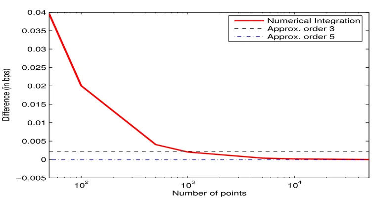
The graph of the error of the numerical integration in term of the number of points is given in

2. The figure represent the difference in price between the different approaches. The second order approximation perform in a similar way to the 1000 points integration.

In term of speed one expect the numerical scheme to perform worst than the explicit (approx-imated) results, at least with enough points. Also the more precise appoximation requires more terms and should be slower. Those expectations are verified in practice. What is maybe not di-rectly expected is the fact that there is an amount of computation required before starting the valuation is-self which is not negligeable. That time is mainly spend in computing the dates and accrual factors (using calendars and market conventions) of the swap. The results are graphed in Figure3.

5. Conclusion

102 103 104 −0.005

0 0.005 0.01 0.015 0.02 0.025 0.03 0.035 0.04

Number of points

Difference (in bps)

Numerical Integration Approx. order 3 Approx. order 5

Figure 2. Convergence of the numerical integration. Semi-logarithm graph. Number of integration points on the x-axis and difference in bps on the y-axis.

101 102 103 104

0 0.2 0.4 0.6 0.8 1 1.2 1.4 1.6 1.8

2x 10

−3

Number of points

Time

Numerical Int. Approx. order 0 Approx. order 3 Approx. order 5

101 102

7 7.5 8 8.5 9 9.5 10 10.5

11x 10

−5

Figure 3. Speed

the standard approach in CMS where the discounting is written as a function of the swap rate. The result of the approximation is very good with a rate precision of 10−7 _{for the second order} and 10−8_{for the fourth order. For any practical purpose the second order approach is more than} enough precise.

Disclaimer: _{The views expressed here are those of the author and not necessarily those of the}

8 M. HENRARD

References

Brody, D. C. and Hughston, L. P. (2004). Chaos and coherence: a new framework for interest-rate modelling. Proc. R. Soc. Lond. A., 460:85–110. 2

Hagan, P. S. (2003). Convexity conundrums: Pricing cms swaps, caps, and floors. Wilmott Magazine, pages 38–44. 1

Heath, D., Jarrow, R., and Morton, A. (1992). Bond pricing and the term structure of interest rates: a new methodology for contingent claims valuation. Econometrica, 60(1):77–105. 2

Henrard, M. (2003). Explicit bond option and swaption formula in Heath-Jarrow-Morton one-factor model. International Journal of Theoretical and Applied Finance, 6(1):57–72. 3

Henrard, M. (2005). Swaptions: 1 price, 10 deltas, and . . . 6 1/2 gammas. Wilmott Magazine, pages 48–57. 2

Henrard, M. (2006). A semi-explicit approach to Canary swaptions in HJM one-factor model.

Applied Mathematical Finance, 13(1):1–18. 3

Henrard, M. (2007). Skewed Libor Market Model and Gaussian HJM explicit approaches to rolled deposit options. The Journal of Risk, 9(4). To appear. Preprint available at SSRN: http://ssrn.com/abstract=956849. 3,4

Hull, J. C. (2006). Options, futures, and other derivatives. Prentice Hall, sixth edition. 1

Hunt, P. J. and Kennedy, J. E. (2004). Financial Derivatives in Theory and Practice. Wiley series in probability and statistics. Wiley, second edition. 2

Pelsser, A., Pietersz, R., and van Regenmortel, M. (2004). Fast drift-approximated pricing in bgm model. Journal of Computational Finance, 8(1):93–124. 3

Contents

1. Introduction 1

2. Model and hypothesis 2

3. CMS pricing 3

4. Implementation 5

5. Conclusion 6

References 8

Head of Quantitative Research, Banking Department, Bank for International Settlements, CH-4002 Basel (Switzerland)