An interval compositional vehicular traffic model for real time applications

An Interval Compositional Vehicular Traffic Model

for Real-Time Applications

Amadou Gning

, Lyudmila Mihaylova

and Ren´e Boel

1

_{Dept. of Communication Systems, InfoLab21, Lancaster University, United Kingdom}

_{SYSTeMS, University of Ghent, Technologiepark - Zwijnaarde 914, Ghent, Belgium}

Email:

{

e.gning,mila.mihaylova

}

@lancaster.ac.uk, [email protected]

Abstract— This paper proposes an interval approach to vehic-ular traffic flow modeling. The developed interval compositional model (ICM) provides a natural way of predicting traffic flows without the assumption of uniform distribution of vehicles along the road. The model can be used for real-time prediction of traffic flows and can be part of road traffic surveillance and control systems. The approach is flexible and robust and can be used in real-time applications. Its performance is investigated and validated over real traffic data.

I. INTRODUCTION

Modeling traffic motion is of paramount importance both for motorways and urban traffic systems. The traffic mod-els available in the literature can be classified into three groups: macroscopic, microscopic andmesoscopic [1], [2]. Macroscopic models require less computations than the mi-croscopic models and are especially suitable for real-time applications. This is a strong motivation for considering the macroscopic models.

In this work we develop aninterval compositional model (ICM) based on the recent stochastic macroscopic traffic model [3]. The interval model is aimed to be applied in on-line algorithms for robust prediction of the traffic state and for on-line control of the traffic system. One of the challenges when working with real traffic data (e.g., from magnetic loops and video cameras) is that they are noisy, coming only from a very limited set of locations and at discrete points in time. The interval model that we propose describes a set of possible interactions between variables in different segments (cells) of the road by means of interval analysis. Then the local dynamics in each cell is obtained by using interval arithmetic in contrast to the point model developed in [3].

Advantages of the proposed approach compared with other approaches are: i) it can take into account the prior information for the allowed intervals of the system states and noises: for instance, the minimum and maximum values of the measurements and system noises are usually known in advance;ii) it affords a natural way to include uncertainties and hence gives robust estimates, andiii) the more motivating fact: it works without the strong assumption that vehicles are uniformly distributed in each segment of the road. In fact, for many reasons (e.g., in the presence of convoys of trucks or due to traffic perturbations) different gaps between vehicles can exist. Moreover, recent studies like in [4] and [5] have

shown that interval-based filtering can reach high-level of precision.

The proposed ICM does not assume uniform distribution of the vehicles within segments, in contrast to the re-cently developed compositional stochastic macroscopic traf-fic model [3], or briefly called compositional model (CM). The only assumption is that vehicles are constrained by the safety distance between them. Similarly to the CM, the ICM describes the complex traffic behaviour with forward and backward propagation of traffic perturbations, but the ICM provides lower and upper bounds on these variables rather than providing a stochastic description of the perturbations. The ICM is, just like the CM, suitable for large networks and for distributed processing. The forward and backward traffic perturbations were characterised in [6] through de-terministic sending and receiving functions and piecewise affine relations between the traffic flow and density. In [7], [3]speed-dependentrandom sending and receiving functions are introduced that represent also the evolution of the average speed in each segment.

The remainder of this paper is organised in the following way. Section II presents the theoretical background of the interval analysis methodology. Section III develops a macro-scopic interval-based traffic model. Section IV validates the proposed model over real traffic data. Finally, Section V generalises the results.

II. INTERVALANALYSIS

This section presents briefly the main interval analysis definitions that we need for the derivation of the interval traffic model. A real interval,[x] = [x, x], is defined as a subset of the setRof real numbers, and a box[x]ofRnx _as

a Cartesian product of nx intervals: [x] = [x1]×[x2]· · · × [xn] =×ni=1x [xi]. In this paper, all interval numbers will be denoted by[x], and all boxes by[x]. The underlying concept

of interval analysis is to deal with intervals of real numbers in place of real numbers. For instance, elementary arithmetic operations, e.g., +,−,∗,÷, etc., as well as operations be-tween sets of Rn_{, such as ⊂,⊃,∩, have been extended to} bounded error context. In addition, a lot of research has been performed with the so calledinclusion functions[8], [9]. An inclusion function[f]of a given functionf is defined such that the image of a box[x]is a box[f]([x])containingf([x]). The goal of inclusion functions is to optimise the interval

Li

Segment i

[Ni,k], [vi,k]

[Ni-1,k], [vi-1,k] [Ni+1,k], [vi+1,k]

[Q i-1,k] [Q i,k]

Sensor locations

1 2 i-1 i i+1 n-1 n

Qk,vk Qk, vk

n+1

Fig. 1. Motorway segments and measurement points.[Qi]is the interval

number of vehicles crossing the boundary between segmentsiandi+ 1, [Ni]and [vi]are respectively the interval number of vehicles and speed

within segmenti.

enclosing the image set and then to decrease the pessimism when intervals are propagated.

The interval framework is well suited for applications to vehicular traffic models since, in practice, lower and upper bounds are known on the measurements errors. This information is quite useful for predicting the traffic flow variables.

III. COMPOSITIONAL MACROSCOPICMODELUSING

INTERVALANALYSIS

The motorway network is modeled as a sequence of segments (Fig. 1). Each segment may contain several lanes in one direction and is big enough to assume that in between two consecutive state update steps of the model no vehicle can cross more than one segment boundary.

Based on all the incoming information, up to the current time, transmitted by sensors to the estimator, traffic states can be estimated at discrete time instants t1, . . . , tk, . . ., possibly asynchronously. The overall state box [x_k] =

([xT

1,k], . . . ,[x T

n,k])at timetk consists of local state vectors [x_i,k] = ([N_i,k],[v_i,k])T, where[N_i,k]is the interval number of vehicles in segment i ∈ I = {1,2, . . . n}, and [vi,k], [km/h], are their interval average speeds. The traffic state evolution is described by the system of equations

[x_1,k+1] = [f1]([Qin_k ],[vin_k ],[x_1,k],[x_2,k]),

[x_i,k+1] = [f_i]([x_i

−1,k],[xi,k],[xi+1,k]), (1)

[x_n,k+1] = [f_n]([x_n

−1,k],[x_n,k],[Qout_k ],[v_kout]), where the function fi is specified by the traffic model; [Qin

k ] is an interval number of vehicles entering segment 1 (interval inflow) during the interval ∆tk =tk+1−tk with an interval average speed[vin

k ].[Q out

k ]is the interval outflow leaving a ‘fictitious’ segmentn+ 1, with an interval average

speed [vout

k ]. Note that [Q in k ], [v

in

k ], and [Q out k ], [v

out k ] are respectively, the interval inflow and outflowboundary vari-ables. They are supplied by the traffic detectors as boundary conditions for the chain of interconnected segments. A. Notations

Let us denote [Di,k_{] the interval virtual distance of a} vehiclec in celli at timek(see Fig. 2)

[Di,k_{] =A}

ℓ+ [vi,k]td, (2) whereAℓ is the average length of the vehicles,[vi,k]is the interval average speed in celliat timekandtd is a constant representing the safe time distance between two vehicles.

Cell i

Virtual distance

_[

_]

d k i l k

i _{A v t}

D, _{= + ,} l

A

Fig. 2. Average virtual distance of each vehicle in cell i

Cell i Cell i+1

Cell i+1 Cell i

(a)

(b)

Maximum empty distance

empty distance = 0

Fig. 3. Calculation of the interval of possible empty space between a convoy of vehicles in cell i: (a) the maximum empty space without considering the virtual distances of vehicles in cell i; (b) when there is no empty distance

Let us denote [Nmax

i,k ] the interval of maximum number of vehicles that can be in the celliat timetk.

[Nmax

i,k ] = (Liℓi,k)/[Di,k], (3) whereLi is the length of celli,ℓi,k is the number of lanes of celli at timek.

Let us introduce[D∆tk

in [vi,k]. Consider then [D Ni,k

k ] the interval of possible empty space between a convoy of vehicles: an interval between 0 and the maximum empty space in cell i without considering the safety distances and the vehicle lengths (see Fig. 3).

[DNi,k

k ] = [0, Liℓi,k−((Ni,k−ℓi,k)Di,k+ℓi,kAℓ)]. (4) To understand this equation (4), Liℓi,k represents the total space available in celli at time k and(Ni,k−ℓi,k)Di,k+

ℓi,kAℓ represents a minimum sum of the virtual distances occupied by, at least,Ni,k vehicles in cell i.

B. Interval Sending and Receiving Functions

The intervalsending function[Si,k]represents the vehicles that “can possibly leave” segmentiwithin∆tk. The interval [Si,k], for each segmenti, having lengthLi, is calculated by

[Si,k] =

ℓi,k[D∆i,ktk]−[D Ni,k k ]

[Di,k_] (5)

The interval [Si,k] is then obtained by calculating the interval distance that can be covered by vehicles in the next cell and by dividing this interval by the virtual distance of vehicles.

The interval receiving function [Ri,k] (6) expresses the maximum number of vehicles that are allowed to enter segmenti+ 1.

[Ri,k] = [Nimax+1,k]−[Ni+1,k] + [Qi+1,k], (6) where [Qi+1,k] is the interval number of vehicles leaving segmenti+ 1(depending on the two intervals[Si+1,k] and [Ri+1,k]). In the next section the calculations of [Qi,k] as well as [vi,k+1] and[Ni,k+1]are detailed.

C. Interval Models for Time Update

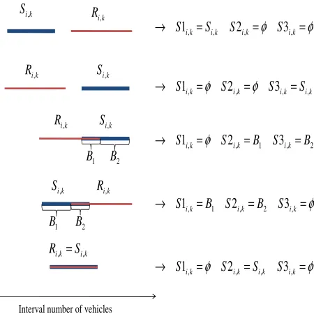
Depending on the position of [Si,k] in comparison with [Ri,k], [Qi,k] can take different values. Let us introduce the partition of [Si,k] into the three sets [S1i,k], [S2i,k] and [S3i,k] (see Figure 4 for illustration of the different configurations) such that:

[S1i,k] =

©

s∈[Si,k]|s < Ri,k

ª

, (7)

[S2i,k] = [Si,k]∩[Ri,k], (8) [S3i,k] =©s∈[Si,k]|s > Ri,kª. (9) For i ∈ {1,2, . . . n−1}, the calculation of the interval outflow [Qi,k] from segment i into segment i+ 1 is given by Algorithm 1. The most complicated case where the two intervals [Si+1,k] and[Ri+1,k]) have an intersection can be interpreted as:

• When the sending functions are in the set [S1i,k], all possible receiving functions are superior to them. Then

[Qi,k] is supposed to be equal to[S1i,k].

Interval number of vehicles k

i

S,

k i

S_,

k i

S,

k i

S,

k i

R,

k i

R_,

k i

R,

k i

R,

k i k i S

R, = , 1 B

1 B

2 B

2 B

φ

φ

= =

→ S1_i,k S_i,k S2_i,k S3_i,k

k i k i k i k

i S S S

S1_, = 2_, = 3_, = _,

→

φ

φ

φ

φ

=

→ S1i,k S2i,k Si,k S3i,k

φ

= =

=

→ S1_i,k B₁ S2_i,k B₂ S3_i,k

2 , 1 ,

, 2 3

1 S B S B

S_ik= _ik= _ik=

→ φ

Fig. 4. The left part of the Figure shows the different configurations for the interval sending and receiving functions. The right part shows the partition of the sending function. HereB1andB2represent different proportions of the sending and receiving functions.

• When the sending functions are in the set [S3i,k], all possible receiving functions are inferior to them. Then,

[Qi,k]is supposed to be equal to[Ri,k]and the average velocity[vi,k] of the[Ni,k] vehicles must be decreased between the two steps according to

[vi,k+1] =ψi([Ni,k],[Ri,k]) (10) whereψiis a function of several parameters (number of lanesℓi,k and lengthLiof the celli, time∆tk between two steps, safe time distancetd between vehicles, etc.). For the choice of ψi we propose to use an analytic inversion of (5). This equation can be written: Si,k in [Si,k]ifSi,kverifies (11), whereα∈[0,1]andD

Ni,k

k =

Liℓi,k−((Ni,k−ℓi,k)Di,k+Aℓ)

Si,k=

ℓi,kvi,k∆tk−αD Ni,k k

Aℓ+vi,ktd

. (11)

From (11), the expression (12) of vi,k can then be obtained, after a straightforward calculation. When re-placing a valueSi,k of the sending function by a value

Ri,kof a receiving function, and withαvarying in[0,1], one obtains a set of values of the average speed

vi,k=

αℓi,kLi+1+Si,kAℓ−αNi,kAℓ

ℓi,k∆tk+α(Ni,k−1)td−Si,ktd

(12) reaching the sending functions equals toRi,k.

Algorithm 1. Interval outflow between celliandi+ 1.

FOR i=n . . .1

IF Si,k< Ri,k, [Qi,k] = [Si,k],[vi,k+1] = [vi,k]

ELSEIF S_i,k> Ri,k,

[Qi,k] = [Ri,k],[vi,k+1] =ψi

`

[Ni,k],[Qi,k]

´

ELSE

[S2i,k] = [Si,k]∩[Ri,k], [S1i,k] =

h

Si,k, S2i,k

i ,

[S3i,k] =

ˆ

S2i,k, Si,k

˜

IF [S1i,k] =∅,

[Q1i,k] =∅,[v1i,k+1] =∅ ELSE

[Q1i,k] = [S1i,k],[v1i,k+1] = [vi,k] END

IF [S3i,k] =∅,

[Q3i,k] =∅,[v3i,k+1] =∅ ELSE

[Q3i,k] = [Ri,k],[v3i,k+1] =ψi

`

[Ni,k],[Q3i,k]

´

END

IF [S2i,k] =∅,

[Q2i,k] =∅,[v2i,k+1] =∅ ELSE

[Q2i,k] = [S2i,k], [v2i,k+1] =ψi

`

[Ni,k],[Q2i,k]

´

∪[vi,k+1] END

[Qi,k] = [Q1i,k]∪[Q2i,k]∪[Q3i,k] [vi,k] = [v1i,k]∪[v2i,k]∪[v3i,k] END

END

After modeling the interval outflow boundary and the interval speed average of vehicles, the general state-space description (1) is given by (13) for the evolution of the number of vehicles and (14) for the speed (see [3] for more details). Remark that the model isexact for the number of vehicles. Concerning the speed, the value (14) comes from a mixture between a predicted speedvinterm

i,k+1 in the cell and an

antic-ipating speedve_(ρantic

i,k+1)depending on the density in front. Ni,k+1=Ni,k+Qi−1,k−Qi,k (13)

          

         

vinterm i,k+1 =

(vi−1,kQi−1,k+vi,k(Ni,k−Qi,k)

Ni,k+1 , for Ni,k+16= 0,

vf, otherwise,

vinterm

i,k+1 = max(vi,kinterm+1 , vmin)

ρi,k+1= Ni,k+1/(Liℓi,k+1) ρantic

i,k+1= αρi,k+1+ (1−α)ρi+1,k+1

vi,k+1= βk+1vi,kinterm+1 + (1−βk+1)ve(ρantici,k+1) +ηvi,k+1

(14) where

βk+1=

(

βI_{, if |ρ}antic

i+1,k+1−ρantici,k+1| ≥ρthreshold,

βII

otherwise.

By using the interval analysis arithmetic and particularly the inclusion functions, the state variables can be easily predicted.

D. Supplementary constraints

By means of the interval analysis the following constraints are added in order to reduce the size of intervals.

1) In each celli, the number of vehicleNi,kat timekand the corresponding average speedvi,kshould satisfy the condition: the total stretch of the road occupied by the vehicles is less than the lengthLi,k of cellitimesℓi,k the number of lanes, i.e.

((Ni,k−ℓi,k)Di,k+ℓi,kAℓ)< Liℓi,k (15) Please note that, this constraint is relevant since the model (14) for the speed can possibly introduce in-consistencies betweenNi,k andvi,k.

2) A second constraint can be introduced, considering the interaction between two neighbouring cellsiandi+ 1. Indeed, the interval outflow boundary [Qi,k] can be interpreted by the fact that the vehicles Qi,k−Q_i,k can be both in cell i and cell i+ 1. Neglecting the uncertainty on the location of these vehicles can lead to false estimations: for instance, in the following steps

k+1,· · ·, these vehicles can be present to the celli+1. For celli, at timek, let us partition Ni,k according to [Ni,k] = [Ni,kR]∪Buf(Ni,k) (16) where [NR

i,k] is the interval of remaining vehicles considering the maximum outflow boundary Qi,k and Buf(Ni,k) is a buffer gathering the vehicles

Qi,j−Q_i,j from the previous steps that are assumed to possibly belong to both celli and celli+ 1. Algorithm 2 describes this decomposition of Ni,k when the sending function [Si,k+1], for the next step k+ 1is calculated. The interval[Ni,k] is replaced by [NR

i,k] and information about the distance covered by the vehicles is used to decide if a group of vehicles in

Buf(Ni,k)can be considered to be in celli+ 1. Algorithm 2. Introduction of a buffer in each cell.

INITIALISATION FOR i= 1. . . n

[NR

i,0] = [Ni,0] Buf(Ni,0) ={∅} Dist(Ni,0) ={∅} END

FORk= 2. . .

USE Algorithm 1 applied to[NR i,k]

FORi= 2. . . n

SUBTRACT[D∆tk

i,k ]from all elements

of the vectorDist(Ni,k−1),

FOR all negative elements ofDist(Ni,k−1)

ADD the corresponding element inBuf(Ni,k)toNi,k+1 SUBTRACT the corresponding element

inBuf(Ni,k)fromNi,k

END

NB

i,k=Qi,k−Q_i,k

DistB i,k=D

Ni,k

k

ADDNB

i,k at the end ofBuf(Ni,k−1)

to obtainBuf(Ni,k)

ADDDistB

i,kat the endDist(Ni,k−1)

to obtainDist(Ni,k)

To illustrate Algorithm 2, we consider an example with two cells. Let assume that at time instantk= 2we have:[N1,2] =

[8,10],[N2,2] = [15,20]; the outflows from cell 1 and 2 are

equal respectively to [Q1,2] = [5,10] and[Q2,2] = [10,20].

By introducing a buffer in each cell, the valueBuf(N1,2) =

5can be calculated. After a period of time where the distance

DN1,2

2 (see III-A and Fig. 3) has been covered in the cell 2,

the vehiclesBuf(N1,2)can be assumed to be out of cell 1.

Then, we must subtract these vehicles from the maximum number of vehicles in cell 1 and add the same number to the minimum number of vehicles in cell 2 (there is an assumption here that the length of cell 2 is bigger thanDN1,2

2 and then

these vehicles are still in cell 2).

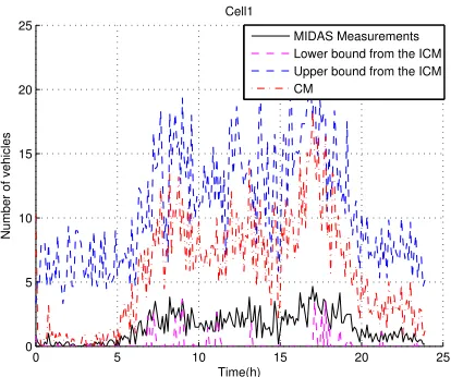
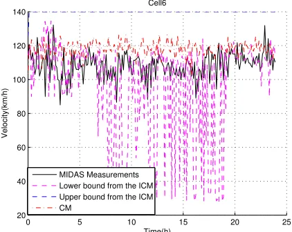
IV. MODEL VALIDATION

The ICM is validated over MIDAS [10], real traffic data sets from the United Kingdom, from motorway M6 (we choose randomly the day 04 September 2002 from data we have). We consider cells 1, 4 and 6 and we plot successively the number of vehicles and the speed. The CM and ICM parameters are chosen in the same way as in [11].

0 5 10 15 20 25

0 20 40 60 80 100 120 140

Cell1

Time(h)

Velocity(km/h)

MIDAS Measurements Lower bound from the ICM Upper bound from the ICM CM

Fig. 5. The Figure shows the evolution of interval velocity boundaries of the cell 1, in relation to the time, given by the ICM (-.), the evolution given by the CM (solid) and the MIDAS measurement (bold).

A stretch from the motorway is considered consisting of eight cells, with three lanes and each having length0.5km. The goal is then, by giving the inflow at cell 1 and the outflow at cell 8, to evaluate the states at all the 8 cells.

In order to validate the performance of the ICM, interme-diate measurements are also shown on the figures, just for comparison. Traffic flows and velocities are calculated for all cells (from 1 to 8) but only the results for cells 1, 4 and 6 are shown due to the lack of space.

Figures 5, 7 and 9 show the evolution of the velocity in cells (1, 4 and 6). Figure 6, Figure 8 and Figure 10 show the evolution of the number of vehicles in these same cells (1, 4 and 6). We can see that the intervals are coherent both with the measurements and the CM simulations (the interval contains the solutions most of the time). In addition, even

0 5 10 15 20 25

0 5 10 15 20 25

Cell1

Time(h)

Number of vehicles

MIDAS Measurements Lower bound from the ICM Upper bound from the ICM CM

Fig. 6. The Figure shows the evolution of interval number of cars boundaries of the cell 1, in relation to the time, given by the ICM (-.), the evolution given by the CM (solid) and the MIDAS measurement (bold).

0 5 10 15 20 25

20 40 60 80 100 120 140

Cell4

Time(h)

Velocity(km/h)

MIDAS Measurements Lower bound from the ICM Upper bound from the ICM CM

Fig. 7. The Figure shows the evolution of interval velocity boundaries of the cell 4, in relation to the time, given by the ICM (-.), the evolution given by the CM (solid) and the MIDAS measurement (bold).

the CM gives good result in comparison with the MIDAS measurements, with the assumption of uniform distribution of vehicles.

However the results obtained for the velocity are better in cell 1 in comparison with cells 4 and 6. The reason is that the velocity given by the inflow measurement, available in this cell, ameliorates the accuracy of the interval boundaries. In contrast, in cells 4 and 6, we see that the lower bound contains several peaks and the upper bound is equal to 140

km/h (this value corresponds to the maximum speed we allowed to the vehicles).

0 5 10 15 20 25 0

5 10 15 20 25 30 35

Cell4

Time(h)

Number of vehicles

MIDAS Measurements Lower bound from the ICM Upper bound from the ICM CM

Fig. 8. The Figure shows the evolution of interval number of cars boundaries of the cell 4, in relation to the time, given by the ICM (-.), the evolution given by the CM (solid) and the MIDAS measurement (bold).

0 5 10 15 20 25

20 40 60 80 100 120 140

Cell6

Time(h)

Velocity(km/h)

MIDAS Measurements Lower bound from the ICM Upper bound from the ICM CM

Fig. 9. The figure shows the evolution of interval velocity bound-aries of the cell 6, in relation to the time, given by the ICM (-.), the evolution given by the CM (solid) and the MIDAS measurement (bold).

are related to the possible numbers of vehicles in the cell. In order to ameliorate these values, the ICM could be refined, by introducing new constraints. For example, when calculating the sending function of a cell i, according to (16), [NR

i,k] (representing vehicles in [Ni,k] that are not in the buffer

Buf(Ni,k)) are considered. One supplementary constraint that can be incorporated too is when the sending function is calculated without the outflow from the previous cell

[QR i₋1,k].

V. CONCLUSIONS

This paper proposes an interval macroscopic model for predicting vehicular traffic flows. Measurements (counts of vehicles and speed) are received only at boundaries between some segments. We demonstrate the feasibility and flexibility of the approach over real traffic data. The proposed interval compositional model can be useful for traffic flows prediction

0 5 10 15 20 25

0 5 10 15 20 25 30

Cell6

Time(h)

Number of vehicles

MIDAS Measurements Lower bound from the ICM Upper bound from the ICM CM

Fig. 10. The figure shows the evolution of interval number of cars boundaries of the cell 6, in relation to the time, given by the ICM (-.), the evolution given by the CM (solid) and the MIDAS measurement (bold).

based on measurements only at some boundaries between segments.

Future research will be focused on testing this interval approach jointly with particle filtering techniques for road monitoring and control purposes.

Acknowledgement. The authors acknowledge the UK Highway Agency and the UK Department for Transport, including Mr William Spurr and Mr Ian Adie for providing us with the real traffic data. We are thankful the EPSRC for the support under project EP/E027253/1.

REFERENCES

[1] D. Helbing, “Traffic and related self-driven many-particle systems,”

Review of Modern Physics, vol. 73, pp. 1067–1141, 2002.

[2] S. Hoogendoorn and P. Bovy, “State-of-the-art of vehicular traffic flow modelling,”Special Issue on Road Traffic Modelling and Control of

the Journ. of Systems and Control Eng. Proc. of the IME. I, 2001.

[3] R. Boel and L. Mihaylova, “A hybrid stochastic framework for real-time freeway traffic modelling,”Transportation Research B

Method-ological, vol. 40, no. 4, pp. 319–334, 2006.

[4] A. Gning and P. Bonnifait, “Constraints propagation techniques on intervals for a guaranteed localization using redundant data,”

Auto-matica, vol. 42, no. 7, pp. 1167–1175, 2006.

[5] F. Abdallah, A. Gning, and P. Bonnifait, “Adapting particle filter on in-terval data for dynamic state estimation,” inProc. of the International

Conf. on Acoustics, Speech, and Signal Processing., 2007.

[6] C. Daganzo, “The cell transmission model: A dynamic representation of highway traffic consistent with the hydrodynamic theory,”

Trans-portation Research B, vol. 28B, no. 4, pp. 269–287, 1994.

[7] R. Boel and L. Mihaylova, “Modelling freeway networks by hybrid stochastic models,” inProc. of the IEEE Intelligent Vehicle Symposium. Parma, Italy, 2004, pp. 182–187.

[8] L. Jaulin, M. Kieffer, O. Didrit, and E. Walter, Applied Interval

Analysis. Springer-Verlag, 2001.

[9] G. Alefeld and J. Herzberger,Introduction to Interval Computations. Academic Press, 1983.

[10] Highways Agency. UK Department for Transport, “Midas: UK road traffic data.” 2007. [Online]. Available: http://www.midas-data.org.uk/, http://badc.nerc.ac.uk/data/ukmo-midas/