A study of the behaviour of multi storey coupled shear walls

A study of the behaviour of multi-storey coupled shear

walls.

TWIGG, David R.

Available from Sheffield Hallam University Research Archive (SHURA) at:

http://shura.shu.ac.uk/20463/

This document is the author deposited version. You are advised to consult the publisher's version if you wish to cite from it.

Published version

TWIGG, David R. (1976). A study of the behaviour of multi-storey coupled shear walls. Masters, Sheffield Hallam University (United Kingdom)..

Copyright and re-use policy

* j act-UNic LIBRAR POND STREET SHEFFIELD Si 1WB

LIBRARY S E R V IC t

M AIN LIBRARY

,.

ghetf,e

ProQuest Number: 10701110

All rights reserved INFORMATION TO ALL USERS

The quality of this reproduction is dependent upon the quality of the copy submitted. In the unlikely event that the author did not send a com plete manuscript and there are missing pages, these will be noted. Also, if material had to be removed,

a note will indicate the deletion.

uest

ProQuest 10701110

Published by ProQuest LLC(2017). Copyright of the Dissertation is held by the Author.

All rights reserved.

This work is protected against unauthorized copying under Title 17, United States C ode Microform Edition © ProQuest LLC.

ProQuest LLC.

789 East Eisenhower Parkway P.O. Box 1346

A STUDY OF THE BEHAVIOUR

OF

MULTI-STOREY COUPLED SHEAR WALLS

A Thesis presented for the CNAA Degree of MASTER OF PHILOSPHY

for research conducted in the Department of Civil Engineering

at

Sheffield City Polytechnic

by

DAVID RONALD TWIGG

ABSTRACT

This thesis deals with the elastic analysis of

non-uniform coupled shear wall structures.

The main methods of analysis available for coupled

shear walls, namely the wide column frame method, the

continuous connection method and the finite element method,

are discussed. Particular attention is given to

non-uniform walls, non-rigid foundations, the importance of

beam-wall flexibility and the importance of coupling action.

The direct solution of the governing differential

equation, derived using the continuous connection approach,

is briefly outlined for a uniform structure, but since the

equations involved very soon became unmanageable when the

method is extended to cater for non-uniform walls, a

numerical solution in the form of the Matrix Progression

Method is studied with a view to using it for complicated

structures. The method is first applied to a uniform

coupled shear wall containing one band of openings and

subjected to both a uniformly distributed lateral load and

a point load. The analysis is then extended to deal with

structures having abrupt changes in geometry and containing

more than one band of openings. A brief description of the

Matrix Progression solutions are presented for a

variety of non-uniform coupled shear walls, including walls

of varying degrees of coupling action supported on both

central and offset columns, and the results are compared

with wide column frame solutions. In addition, for both

symmetrical and non-symmetrical walls with one abrupt change

in cross-section, the solutions are compared with

ACKNOWLEDGEMENTS

The author is greatly indebted to Professor A Coull

of Strathclyde University for his supervision, guidance

and encouragement during the later stages of the work, to

Dr R D Puri for suggesting the work and his supervision

during the initial stages, and to Mr P Ahm and his

colleagues at Ove Arup and Partners for interesting

discussions on the practical problems of shear wall design. i

Sincere thanks are due to all members of the Civil

Engineering Department at Sheffield City Polytechnic who

have given help during the period of the work.

The author also wishes to thank Miss J Bradley for her

careful typing of the thesis.

-CONTENTS

Page

CHAPTER 1 INTRODUCTION 1

1.1 Introduction 1

1.2 Past Work 2

1.3 Scope of Present Work 15

CHAPTER 2 ANALYTICAL SOLUTION 17

2.1 Introduction 17

2.2 Notation _ * 17

2.3 Assumptions 18

2.4 Uniform Coupled Shear Wall ' 19

Containing One Band of Openings

2.5 Complex Shear Wall Systems 25

CHAPTER 3 MATRIX PROGRESSION SOLUTIONS 27

3.1 Introduction 27

3.2 Notation 29

3.3 Assumptions 30

3.4 Uniform Coupled Shear Walls 30

Containing One Band of Openings

3.5 Coupled Shear Walls Containing 43

One Band of Openings and with One Abrupt Variation in Cross-Section

3.6 Uniform Coupled Shear Walls 49

Containing Two Bands of Openings

3.7 Coupled Shear Walls Containing 56

Two Bands of Openings and with One Abrupt Variation in Cross-Section

3.8 Coupled Shear Walls Containing 59

n Bands of Openings and with m Abrupt Variations in Cross-Section

CHAPTER 4 COMPUTER PROGRAMS

4.1 Introduction 61

Page

CHAPTER 5 EXPERIMENTAL WORK 69

5.1 Introduction 69

5.2 Material 69

5.3 The Models 70

5.4 Method of Test 70

CHAPTER 6 RESULTS 78

6.1 Introduction 78

6.2 Theoretical Results 78

6.3 Results for Walls Containing One 81 Band of Openings and with One

Abrupt Variation in Cross-Section

6.4 Results for Uniform Walls 109

Supported on Columns

6.5 Results for Walls Containing Two 136 Bands of Staggered Openings

CHAPTER 7 DISCUSSION OF RESULTS 140

7.1 Introduction 140

7.2 Walls Containing One Band of 142

Openings and with One Abrupt Variation in Cross-Section

' 7.3 Uniform Walls Supported on Columns 144

7.4 Walls Containing Two Bands of 147

Staggered Openings

7.5 Conclusions and Suggestions for 148 Future Work

REFERENCES 150

-CHAPTER 1

INTRODUCTION

1.1 Introduction

With low rise buildings the primary concern of a

design is to provide an adequate structure to support the

applied vertical loads. In tall buildings, however, the

effect of lateral loads is very significant, from both the

strength and serviceability points of view, and it is

important to ensure adequate stiffness to resist these

lateral loads which may be due to wind, blasts or earth­

quake action.

The required stiffness may be achieved in various ways.

In framed structures it is obtained from the rigidity of

the member connections but when the frame system alone is

insufficient, additional bracing members may be added or,

as is more usual, reinforced concrete 1 shear walls* are

introduced. The term ‘shear wall* can cover stair wells,

lift shafts and central service cores but in the present

work it is used to denote plane walls in which the high in­

plane stiffness is used to resist the lateral forces.

In its simplest form the shear wall consists of a

single cantilevered wall which behaves according to simple

contain openings for doors and corridors but may also

have an abrupt change in cross-section at a certain height

or may even be supported on columns. In such cases the

behaviour of the walls is much more complicated.

The structures considered in the present work are

those comprising shear walls connected by beams which form

part of the wall, or floor slabs, or a combination of both.

1. 2 Past Work

Prior to 1960 little attention was paid to the

development of analytical techniques for shear walls. In

recent years, however, much research has been carried out

and comprehensive reviews of the methods of analysis, and

sources of information on the subject have been presented

by Coull and Stafford Smith (1 and 2) and Fintel et al (3).

The only work which will be mentioned here is that

which is relevant to the work considered in this thesis.

The analysis of walls pierced by sets of openings

(coupled shear walls) has received much attention but as

with any complicated structural system the accuracy of the

analysis is dependent upon the form of idealization given

to the actual structure together with the assumptions that

the idealization involves. Since methods of analysis

involving the solution of the governing plane stress

elasticity equations are difficult to implement in connection

-with coupled shear walls, all the methods of analysis

which have been used previously have involved the idealiza­

tion of the structure as an interconnection of elements of

which the properties are known or can be estimated. The

main methods which have been used are:

(i) frame analogies

(ii) finite element method

(iii) continuous connection method.

Frame Analogies

The first of the frame analogies is the ‘equivalent

frame method1. In this method the walls are replaced by

line members along their centroidal axes and the lengths of

the connecting beams are taken to be the distances between

the resulting line members, thus making the structure a

vertical vierendeel girder (see Figure 1.1(b)). Because in

most cases the width of the walls is not negligible compared

with their centre line distances, this approach is

unrealistic and will generally overestimate the deflections.

Green (4) adopted this procedure and used the ’portal

frame* method of analysis, assuming points of

contra-flexure at the mid-points of all members. Although he

used modified stiffnesses to take account of shear as well

as bending, he neglected axial deformations of the walls

£

Is

•H_4-J O(U G G o a w G o GG •rH_Jj G o u

I 1 I 1 I 1 I 1 I 1

I 1

I I I I I I I I L _ L _

I 1

I--- 1 I 1 r “ i 1

i---i i

i i i____

L _ L _ I__ I I

cd <u § J-i tii

i

§

Figure 1.1 Coupled Shear Wall and Idealized Structures

-An improvement on the ‘equivalent frame method* is \

the so-called ‘wide column frame *. In this method the

length of the beam connecting elements is taken as the

clear distance between adjacent walls and account is taken

of the effect of the vertical deflections at the ends of

the beams, which are due to rotation of the walls, by

assuming that the member joining the beam end to the wall

centre-line is infinitely rigid (see Figure 1.1(c)).

Once the analogous system has been set up, the analysis

is best preformed by using matrix stiffness or matrix

flexibility methods of analysis. Both methods are well

established and documented (e.g. 5 and 6) and standard

computer programs are available, usually adopting the

stiffness approach (e.g. 7 and 8).

Frischmann, Prabhu and Topler (9) used the flexibility

method for the solution of a wide column frame, but as with

Green axial deformations of the walls were ignored.

MacLeod (10) used the stiffness method to obtain a

solution by incorporating stiffness matrices for elements

which have infinitely stiff end sections.

A variation of the above method, allowing standard

computer programs to be used, was presented by Schwaighofer

and Microys (11). They considered the rigid arms as

cross-sectional area and moment of inertia. A disadvantage of

this method, however, is that the number of nodes in the

structure is doubled, thus making much heavier demands on

computer capacity and time.

A further variation for symmetrical structures only

was presented by Stafford Smith (12) who replaced the

rigid-armed beam by an analogous uniform beam with the same

rotational end stiffness. This allowed a standard computer

program to be used without any increase in the number of

nodes.

Finite Element Method

The basis of the finite element method is that any

structure can be considered as an assemblage of individual

elements, of which the properties are known, connected to

each other only at discrete nodes. This is in fact what

has been done in the frame analogies but finite element

analysis usually refers to systems where the elements are

two or three dimensional rather than line elements. The

method is well documented and typical works are by

Zienkiewicz (13) and Rockey et al (14).

Although elements of any shape can be used it is

general, in shear wall analysis, to use either rectangular

or triangular elements with the triangular elements being

of nearly uniform stress and fine meshes in regions of

high stress gradients. One very big disadvantage of the

technique is the large amount of computer storage required

for a solution and because of this the value of the method

lies in the analysis of local stress distributions rather

than an overall analysis of a structure.

Choudhury (15) used the method to make comparisons

with the solutions obtained from other forms of analysis

and MacLeod (10) used the method for the analysis of

coupled shear walls with relatively stiff beams. His work

showed that rectangular elements gave satisfactory results

provided the mesh was not too coarse.

MacLeod (16) also derived a special element having a

rotational degree of freedom at each node and was thus able

to combine line elements in bending, which are needed for

slender connecting beams, with the plane stress elements of

the walls.

Continuous Connection Method

In the ’continuous connection method* the discrete set

of connecting beams, which are usually evenly spaced, is

replaced by an equivalent continuous medium which is

assumed to be rigidly attached to the walls but which is

only capable of transmitting actions of the same type as

the connecting beams have a point of contraflexure at mid­

span and that they do not deform axially, the method leads

to a definition of the behaviour of the system as a second

order differential equation which can be solved for

particular load cases.

Although the replacement of a series of members had

been used before for tall frame buildings by Chitty (17),

Beck (18) appears to have been the first to apply this

method to coupled shear walls when he considered the single

case of two uniform coupled shear walls on a rigid founda­

tion, subjected to a uniformly distributed lateral load.

In the analysis he used the shear forces in the connecting

medium as the statically indeterminate function.

Using the integral of the shear force in the connecting

medium as the indeterminate function, Rosman (19) derived

solutions" for a wall system with one or two symmetric

bands of openings, with various support conditions at the

base of the walls, and for both a uniformly distributed

load and a single point load at the top.

Coull and Puri (20) considered the same problem as

Beck but in their analysis they took account of the shear

deformations in the walls, in addition to the axial and

bending deformations in the walls, and the bending and

shear deformations in the connecting medium. These effects

of shear had been ignored by previous researchers and were

shown not to have a significant effect on the results of

the analysis.

In the design procedure for shear walls put forward by

Pearce and Mathews (21), the basic equations of the continu­

ous connection method were re-written to include the wind

loading shape of CP3 (22). . However, it was concluded that

for practical purposes, satisfactory results could be

obtained by using the formulae for a uniform loading.

The simplicity of the general technique has enabled

Coull and Choudhury to put forward design curves (23 and

24) and Rosman to put forward design tables (25) which

enable a rapid and accurate analysis of the structure for

standard load cases.

Importance of Beam-Wall Flexibility

- In all the analyses outlined it has been assumed that

the beam-wall connection is fully rigid, but due to high

stress intensities at these connections local deformations

will occur which effectively increase the flexibility of

the connecting beams.

Michael (26) analysed these local deformations by

considering the wall as a semi-infinite elastic plane and

the effects of these deformations were calculated as

of the reduction factors with the geometric proportions

of the beam were presented as graphs. He suggested that

for most span to depth ratios likely to occur in practice .

it is possible to take this extra flexibility into account

by assuming an increase in the clear span of the beam of

half its depth on each side.

Further work was done by Bhatt (27) who conducted an

investigation of the local deformations using the finite

element procedure. He concluded that the effect of junction

deformations was only important when the ratio of beam

length to depth was less than 5, and that for ratios

between 5 and 3 the correction suggested by Michael could

be used. For the analysis of walls with stiffer connecting

beams he presented further modifications in graphical and

tabular form which could be applied to both the continuous

connection and wide column frame methods of analysis.

Importance of Coupling Action

When the openings in a coupled shear wall system are

very small their effect on the overall state of stress is

minor. Larger openings have a more pronounced effect and,

if large enough, result in a system in which typical frame

action predominates. The degree of coupling between the two

walls connected by beams has been conveniently expreseed in

terms of the non-dimensional geometric parameter ocH, which

! *

-gives a measure of the relative stiffness of the connecting

beams with respect to that of the walls. The parameter

appears in the basic differential equation of the continuous

connection method.

A study by Marshall (28) indicated that when ©cH

exceeds 13 the walls may be analysed as a single solid

cantilever, and when is less than 0.8 the walls may be

treated as two separate cantilevers. For intermediate

values, the stiffness of the connecting beams should be

considered.

-The question of when coupling action is important was

also considered by Pearce and Mathews (21) and they decided

that the upper limit for c*H should be 16 and that the

lower limit should be 4.

However, despite the difference in the sets of figures

given, it would appear that for most wall systems likely

to occur in practice the coupling action should be

considered.

Non-Uniform Coupled Shear Walls

Because the coupled shear wall system is replaced by

a large number of individual elements in the wide column

frame method, any number of variations in cross-section or

any number of connected walls can easily be accommodated,

However, with the continuous connection method the

algebraic expressions involved only allow a limited number

of discontinuities to be incorporated.

Traum (29) used the continuous connection method to

analyse a system of symmetrical coupled shear walls pierced

by one band of openings and with a single stepped variation

in cross-section and intensity of uniformly distributed

loading. The upper zone of the wall was solved as being

elastically supported on the lower one and that was then

analysed by subjecting it to axial forces, bending moment

and shearing force at its top together with the external

horizontal loading.

Using the same approach, but applying all the loads

simultaneously, Coull and Puri (30) presented a simpler

analysis of the problem considered by Traum but which also

included ’the effects of shearing deformations in the walls.

Pisanty and Traum (31) presented their own simplified

analysis but there seemed to be disagreement between the

two sets of authors as to the conditions to be adopted at

the change in wall section.

Another type of discontinuity was presented by Coull

and Puri (32) who considered a stepped variation in the

thickness of the walls.

To overcome the complexity of analysing shear wall

-systems with more than one abrupt change in cross-section

and/or more than one band of openings by the analytical

procedures (i.e. by direct solution of the governing

differential equations) a numerical approach to the problem

in the. form of a matrix progression solution was presented

by Puri (33).

The essential features of the ’matrix progression

method' are given by Tottenham (34). When applied to

coupled shear wall analysis the basis of the method is that

the structure is divided into uniform zones and differential

equations governing the behaviour of each zone can be

determined. An overall solution is then obtained by

applying boundary and continuity conditions. The only

limitation of the method, when applied to shear walls, is

that the centre line of each band of openings must be

continuous throughout the total height of the wall.

The method was extended by Coull, Puri and Tottenham

(35) to the solution of coupled shear wall systems containing

any number of stepped variations in cross-section and any

number of bands of openings. At the same time the number

of differential equations governing the behaviour of each

zone was reduced, thus lessening the work load required in

an analysis.

only considered walls containing one band of openings but

included the effects of flexible foundations in their

analysis.

Non-Rigid Foundations

Many shear wall systems are rigidly built in at

foundation level but in practice other base conditions can

occur. On one hand the walls may be built on independent

foundations which yield vertically and rotationally relative

to ea.ch other. On the other hand, the walls may be

supported at first floor level on a column system to allow

large open spaces at ground floor level. If either of

these two conditions occur, the behaviour of the lower

parts of the wall system can be significantly altered.

The analysis of walls on flexible foundations using

the wide column frame method presents no problems as most

standard ’computer programs allow prescribed displacements

to be applied at any node.

MacLeod and Green (37) used the wide column frame

method to analyse a wall with one band of openings supported

on a beam and column system. They considered symmetrical

and non-symmetrical walls with both stiff and flexible

connecting beams and they showed that the results obtained

agree satisfactorily with finite element analysis.

The use of the continuous connection method for the

-analysis of walls supported on columns was first put

forward by Rosman (19).

Further work using this method has been done by Coull

and Chantoksinopas (38) who presented design curves for

any pair of walls or a set of three symmetrical walls

supported on any elastic foundation or any beam column

system. Three loading cases, namely a uniformly distri­

buted load, a point load at the top and a triangular load

were considered and a complete solution for any load form

and any base condition can .be obtained using only three

design charts. A comprehensive series of formulae, rather

than charts, for the analysis of similar structures have

also been presented by Coull and Mukherjee (39).

Arvidsson (40) also considered the problem and

presented a method for analysing shear walls with two

bands of openings supported on an elastic foundation.

1.3 Scope of Present Work

Although the continuous connection method is well

accepted for the analysis of uniform coupled shear wall

systems, it has frequently been criticised as not having

the flexibility of the wide column frame method to cover

non-uniform structures. Although this criticism is

justified when the analytical solution is employed, it has

potential for the analysis of complex wall systems if a

numerical solution is adopted.

The object of the present work is to check the

accuracy of the matrix progression solution of the

continuous connection method against both experimental

results and the wide column frame method for a variety of

non-uniform coupled shear walls, including walls supported

on columns.

-CHAPTER 2

ANALYTICAL SOLUTION

2.1 Introduction

In this chapter, the differential equations governing

the behaviour of a uniform coupled shear wall structure

with a rigid foundation are derived using the continuous

connection, and an analytical solution is obtained.

Although the method itself has appeared frequently

before, it was thought necessary to include it here to

show the procedure adopted in the solution, and also as an

introduction to the numerical method presented in Chapter 3.

To achieve consistency with the numerical solution,

the equations have been derived using the base of the wall

as the origin for the x co-ordinate, and in this respect

they differ from previously published equations.

The only loading case considered is that of a uniform

lateral load.

2.2 Notation

The following symbols are used in this chapter.

aA> a b Cross-sectional area of walls A and B respectively

b Length of connecting beams

d Depth of connecting beams

G Shear modulus

H Total height of wall

h Storey height

1^, Ig Moment of inertia of walls A and B respectively

Ig Moment of inertia of connecting beams

Iv Reduced moment of inertia of connecting beams

Q Distance between centroidal axes of walls

M^, Mg Bending moment in walls A and B respectively at a height x

Ma Applied bending moment at a height x

N^, Ng Axial force in walls A and B respectively at a height x

q ... Applied lateral distributed load

VA , V-d Shear force in walls A and B respectively at a

height x

v Distributed shear force in the substitute connecting medium at a height x

x" Height above foundation

y ^ Lateral deflection of walls at a height x

Any other symbols used are defined as they are

introduced.

2.3 Assumptions

(a) The walls have a rigid foundation

(b) The moments of inertia and cross-sectional areas of both the walls and the connecting beams, and the storey height are constant throughout the height of the

structure.

-(c) The points of contraflexure of the connecting beams are at their midspan

(d) The connecting beams do not deform axially and hence the lateral deflection of individual walls is the same at any level

(e) In each zone the discrete set of uniform connecting

beams may be replaced by a uniform equivalent connecting medium of the same stiffness. The stiffness of the

connecting medium for half a storey height above the foundation is considered as taken from the rigid connection at the foundation

(f) Plane sections of the wall before bending remain plane after bending. This allows the moment-curvature

relations based on the engineers theory of bending to be used for individual walls

(g) The beam-wall connection is fully rigid.

2.4 Uniform Coupled Shear Wall Containing One Band of Openings

The structure considered is shown in Figure 2.1,

where the individual connecting beams of stiffness EI^

are replaced by an equivalent continuous medium or

lamellae of stiffness El^/h per unit height.

Governing Differential Equation

Consider a 'cut' along the centre line of the medium

connecting the two walls. There will be movement of the

two parts of the medium due to both rotation and vertical

Figure 2.

—

.. - - I b 1— 1

1 1

— _{a a} 1___ J_{1 1 a r}

— 1 1 %

1 -1 — L_{1 '} J _{i j h}

' 1_____ I ' I

— r n 1

i .'..

777777777777777777777

H

x

Wall A Wall B

7 7 7 7 7 7 7 7 7

/;

77777777777

1 Coupled Shear Wall and Substitute System

- 20 - •

The axial force in wall A at any height x is given

by:

na = H vdx

and thus the vertical movement of wall A at a height x is

given by:

rx

EA,

r H

o J vd^ dx

where is a dummy variable which is used to signify the

variation of within the region 0 to x.

For vertical equilibrium of the wall system

n b ■ -n a

and thus the vertical movement of wall B at a height x is

given by:

rx

EAB

H

vd*k dx

Thus the total relative displacement at the cut is

given by:.

i = 2 §1 _ i ( i + i ) dx E ( Aa Ab )

r x

o J H

?>

dx

To restore continuity in the connecting medium, a

shearing force v must be applied across the cut so that

12EIv S v =

hb'

where Iv is a reduced moment of inertia to take account of

shear and is given by:

Thus the compatibility equation is: H

vd>) dx = 0 (2.1) . I (1 . i ) fX

dx ” 12EXVV " E (Aa + AB ) _{J o >■}

The moment curvature relationship for the walls is:

d2y _ -M dx2 El

where M = + Mg

and I = 1^ + Ig

and thus:

a2

E1~ 2

==

^H"‘X^2" ® j vdx

(

*

)

A differential equation governing the distributed shear

force can now be obtained by differentiating Equation 2.1

w.r.t.x, substituting Equation 2.2 and differentiating

again.

Thus: 2

- <*2V = -2B (H - x) (2.3)

dxz ,i .

where 2 _ 12IV ( ^ , A )

= ( I A * Ar )

and a qQ 1 2IV 1

V = 2 - z z r i

hbJ v A B

121

,

hb3 and where

A = Aa + Ag

Solution for Distributed Shear Force

The general solution of Equation 2.3 is:

v = Peotx + Qe_0O!; + _oC^2 _{(H - x) (2.4)}

where P and Q are constants of integration which depend on

-the boundary conditions.

At the base, the rotation is zero and thus, from

Equation 2.1, we obtain:

v = 0 when x = 0

At the top of the wall, the moment, and thus the

curvature are zero and once again from Equation 2.1 we

obtain:

4— = 0 when x = H_dx

Using the above conditions, Equation 2.4 becomes:

V = F l ( 2 . 5 )

where

1 + £*Hsinh(*H . ( TT x )

F1 = ' c*.Hcosh<xH. Sinh ( * H H ) (2-6)

, ( „ x ) , ( „ x ) -cosh ( <*H 5 ) + ( 1 - ii }

and A T

ft - 1 + A 1 aaab S>2

Height of^ Maximum Distributed Shear Force

From Equation 2.5 it is seen that the maximum value

of the distributed shear force v occurs when is a

maximum.

Thus, differentiating Equation 2.6 w.r.t.x and equating

to zero, the only valid solution for x is

x _ h -l-i ( coshocH + sinhocH - oiH ) ,9

H <*H ge ( coshoOI - sinhoiH'+oiH ) ' }

Equation 2.7 into Equation 2.6 to give F-jmax and then

substituting this value into Equation 2.5.

Axial Force and Bending Moment

The axial force in each wall is given by:

R

N = vdx

x

Substituting Equation 2.5 and re-arranging the terms

we obtain:

“ = ^ 2 ■ (2 .8)

Where Mq = q(H ~ x^2

and „ 2 f l+^Hsinho^H , ( TTx)

F2 = («fl)2( x)2 ) 1 — sh«H ' cosh(^HH) ( H)

<-. it • i ( >,x) , GxH)2 (., x)27

+ o^Hsmh(o<HS) + - j — (l— j J

The moment resisted by the axial forces N is N2, which

McjF 9

from Equation 2.8 is equal to — .... .

h

Thus the moment resisted by bending of both walls is

given by:

M = Mq,l -h

Deflections

M = Mq^l - ^ (2.9)

( |x)

The deflection y at any height can be obtained by

substituting Equation 2.5 into Equation 2.2, integrating

twice w.r.t.x and applying the appropriate boundary

conditions,

-Thus

(

.

)

where

. U . h j s r + I * . ± } j V A (24 ( H) 6 H 24 ) | P )

+

2

(*H)3 ( H)j

For the maximum deflection ymax the condition x = H

can be substituted into the equation for F3 and thus

2.5 Complex Shear Wall Systems

The’method of analysis presented in Section 2.4 can

obviously be extended to cater for any number of bands of

openings and any number of abrupt changes in cross-section.

However, each band of openings produces a differential

equation of second order, and each change in cross-section

requires the solutions of the equations below and above the

discontinuity to be matched. Thus only two, or possibly

three, such effects can be dealt with before the algebraic

expressions involved become unmanageable and it is for qH4 „

ymax = e i" 4

(

.

)

where

this reason that alternative methods of analysis have been

developed.

-CHAPTER 3

MATRIX PROGRESSION SOLUTIONS

3.1 Introduction

The Matrix Progression Method, as outlined by

Tottenham (34), is a technique of structural analysis

especially designed for application to complex structures

composed of several shell or plate elements. The analysis

of these structures involves a considerable amount of

numerical computation whatever method is used and the

purpose of the matrix progression method is to make the

analysis as simple as possible, because by using matrix

algebra the calculations are readily planned.

The basis of the method is a special form of solution

of the basic differential equations governing the stress

and displacement conditions in a structure. The solution

is in two parts, corresponding to the complementary function

and the particular integral, the first part of which depends

only on the boundary conditions at one end of the structure

and the second part of which depends only on the loading

system. By using the solution in this form we can write

the solution for an element of the structure in general

terms and add in the effects of applied loads, or changes

The essential requirements of the method are that the

sum of the order of the basic differential equations must

be even, and one half of the boundary conditions must be

known at each end.

In this chapter, a uniform coupled shear wall contain­

ing one band of openings and subjected to both a uniformly

distributed load and a point load is considered first. The

analysis is then extended to deal with systems in which an.

abrupt change in geometry of the structure takes place at

a particular height. This is done by splitting the structure

into two zones such that the geometric properties and

applied loading intensity remain constant in any one zone.

The only restriction to the variation of the geometric

properties and loading from one zone to the other is that

the line of the centres of the connecting beams is continu­

ous through the two zones. Sets of differential equations

governing the behaviour of each zone are determined and a

solution is obtained by.applying appropriate continuity and

boundary conditions.

The solution is then extended to deal with structures

containing two bands of openings and having an abrupt change

in cross-section, and finally the analysis is generalised

for coupled shear walls with any number of bands of

openings and any number of abrupt variations in cross-section.

/

-3.2 Notation

The following symbols are used in this chapter:

AA ’ a b Cross-sectionai area of walls A and B respectively

aN,A> aN,B Axial displacement of walls A and B respectively at a height x

B^, Bg Width of wall-s A and B respectively

Length of connecting beams

Depth of connecting beams

Young *s modulus

Applied point load

Shear modulus

Total height of wall or zone

Storey height

Ia > Ig Moment of inertia of walls A and B respectively

Ig Moment of inertia of connecting beams

Iv Reduced moment of inertia of connecting beams

J Distance between centroidal axes of walls

M^, Mg Bending moment in walls A and B respectively at a height x

^A» ^B Axial force in walls A and B respectively at a height x

q Applied distributed load

VA , Vg Shear force in walls A and B respectively at a height x

v Distributed shear force in the substitute

x Height above foundation or discontinuity

y Deflection of walls at a height x

0 Rotation of walls at a height x

. The additional suffices 1 and 2 after any symbol

refer to zones 1 and 2 respectively.

Matrices are denoted by underlining the symbol e.g. A,

Any other symbols used are defined as they first

appear.

3.3 Assumptions

The assumptions made are the same as in Section 2.3

except that (a) need not apply.

3.4 Uniform Coupled Shear Walls Containing One Band of Openings

The coupled shear wall system referred to in the

following analysis is shown in Figure 3.1.

Displacement and Elasticity Relationships

At any distance x from the base, the lateral displace­

ment y and the rotation 0 are equal for both the walls and

their relationship is given by:

. £ " <3-1)

Consider now a *cut* along the centre line of the

medium connecting the two walls. There will be a movement

of the two parts of the medium due to both rotation and

vertical movement of the walls (See Figure 3.2).

-F igure 3.

—

&x and £>

777777777777777777777

a

Wall A Wall B

Figure 3.

■ - ) — 4

-A~

1

-aN, A _{aN JB"}

_| —

2 Displacement of the ends of the cut connecting medium

-The end attached to wall A will approach the base by

an amount b

^2 + ~ aN,A

while the end attached to wall B will move away from the

base by an amount *

b

( 2 + — ) e + aN,B

The relative displacement at the cut, 8 , is thus

f

given by

8 =

a.

To restore continuity’in the connecting medium, a

shearing force v must be applied across the cut.

The deflection of a unit cantilever due to bending and

shear is given by

s =

v

12EIV

where Iv is a reduced moment of inertia to take account of

shear force and is given by

_ ib

Iv " 1+1 .2WG ('Vb) 2

Thus the value of the shear force is given by

V = T 5 T ( Je " aN.A + aN,B> (3-2)

The moment-curvature relationship for the walls is

i= -if

' <3-3>

The vertical strain of the centre line of wall A is

A an(j j_s given by dx

daivr a N a

- ^ - ^ = _dx 7 7_EA^ (3.4)_{' 7}

Similarly

daN,B % ,,

dx EAb V ;

Diffentiating Equation 3.2, and substituting Equations

3.3, 3.4 and 3.5, we obtain

dv ■ 12IV ( M5 % % ) ,

dx ( " I AA + AB ) ^ ’b>

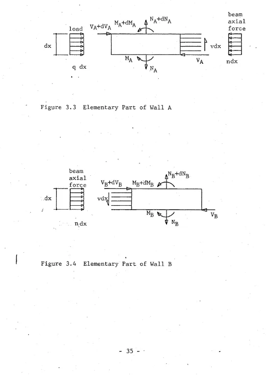
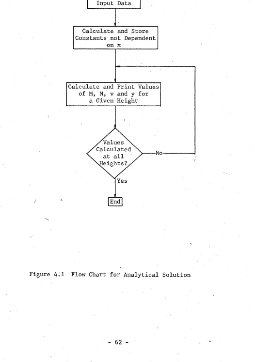
Equilibrium Conditions

Consider an elementary part of wall A of height dx as

shown in Figure 3.3.

For vertical equilibrium

dNA

' dx = -v * (3.7)

^For moment equilibrium, ignoring the second order

derivatives

dMA (2A . b ) . _ /q n\

d F = 'v ( 2 + 2) + VA (3-8)

Consider now an elementary part of wall B of height

dx as shown in Figure 3.4.

dN-r>

d T = v <3 -9>

-dx

q dx

*

vdx

beam axial force

ndx

Figure 3.3 Elementary Part of Wall A

dx

beam axial

orce

---ndx

ANB+dNB

Vg+dVg Mg+dMg pr~ ^

--- &>i---vdx

MB

V N_B 'B

For moment equilibrium, once again ignoring the second

order derivatives

<J

mb

(b

bb

)

1f.|

“djT “ " v ( 2 T ) B (3-10)

Combining the moment equations 3.8 and 3.10 gives

^=-2v + V '

(3.11)

where V = + Vg

For vertical equilibrium of the wall system it is

required that

Ng =

-N

a

(3.12)

and substituting Equation 3.12 into Equation 3.6 gives

dv _ -12Iv j) _ 12IV (1 1

)N

a

or

where

and

g = + FlNa (3.13)

-121, Y " -v

hb3I

-1 2IV (1 . 1 ) hb3 (aA Ab )

For horizontal equilibrium of the wall system

g = - q (3.14)

System of Equations

In Equations 3.1, 3.3, 3.11, 3.14, 3.13 and 3.7 we

have obtained a set of six first order differential

equations containing the actions y, 0, M, V, v and N^. If

-we now express these equations in terms of a non-dimensional

height co-ordinate ^ where

% = _H

we obtain = d S dO dM d S dV d^ dv H0 ,M

"h'ex

= -H « v + HV

= -Hq

^ = H tfM + H f*NA

d %

d % = -Hv

and these equations can be expressed in matrix form as

Ey EG M V V na

0 H 0 0 0 0

0 0 "H/i 0 0 0

0 0 0 H -Hfi 0

0 0 0 0 0 0

0 0 Hy 0 0 Hp. 0 0 0 0 -H 0

Ey ₊ 0

E0 0

M 0

V -Hq

V 0

n a 0

which can be written as

d S

-r-f_{d S} 1 = A S + B_{_ _ _} (3.15)

A = H 1 0 0 0 0 0 0 0 - 1 VI 0 0 1

0

0

Jf 0

0 0 0 0 -a 0 0 1 0 0 0 0 K 0

and _{B = |0 0 0 -Hq 0 0 1 T}

Solution of Equations

Equation 3.15 is a linear first order differential

equation and the integrating factor required for its

solution is

- 1 / a - \-l ( [a de ) _ 1 _ ( At ) (e J ) " (e ’ )

Multiplying the equation by this factor gives

( A O - i d j J i ) ( a O - 1 a s ( a O - 1 b

(e ) (e ) VV (e )

-which reduces to

(5 )| _ ( e ^ ) - l B «

Integrating,we obtain

( e M) ' 1 S (§) = - A" 1 ( e M) " 1 B + K (3.16)

where K is a constant of integration.

Substituting the boundary condition of

£ (^) = £ (0 ) when £ = 0

gives

K = S (0) + A"1 B

Substituting this value of K into Equation 3.16 gives

S(«=) = e£% S(0) - A-1 B (3.17)

Now eA§ _ I + A£ ' + - 2 *>2 + - 3 ^ 3 + ___

~ 21 31

Thus ,

2

2

1 I • • • •

- = A 6,

21 3!

and so

- A" 1 B = fl^ + ~ ^ 2 + - % + ____ ^ B

Equation 3.17 can now be written as

S(§) = G(|) S(0) + F(fp (3.18)

where ^ „

a £ A3 £ 3

G ( 0 = I + A £ + - ?. + ~ 5 + ....

“ 21 31

and /• a <- 2 a2 ^ 3

£ < S>- | i 5 * ^ - + =j^ + ....]b

Boundary Conditions

At the base of the wall, i.e. when £ = 0, the displace­

ments y,■ ”&n,A and aN,B> anc^ rotation 0 are all zero

and by substituting the value of v as zero. Thus

yo = o

e0 = o

vQ = o

These boundary conditions can be used to express the

action matrix S_(0) in terms of the matrix Sp which contains

only the unknown conditions at the base i.e. M0 , V0 and N0 .

Thus

where

0 0 0 ,

0

0

0

1 0 0

0 1 0

0

0 . 0

0 0 1

M0 V0 N0

If the base is not fixed but is capable of rotation

and vertical settlement then the forces and displacements

at the base are related by

Yo = 0 0 0 _M0

e

0

v

0

where C^, C3 and C3 are constants dependent upon the

rotational stiffness and the vertical displacement stiffness

of the base and thus the value of K0 in Equation 3.19 is

given by

0 0 0

Cl 0 0 1 0 0

0 1 0

c2 0 C3

0 0 1

K0

and

S0

-By substituting Equation 3.19 into Equation 3.18 we can

write the solution of Equation 3.15 as

£(§)=£($) Ko S0 + F(|=) (3.20)

. Thus at the top of the wall, i.e. when £, = 1

S(l) = 6(1) K0 S0 + F(l) (3.21)

Now at the top of the wall, the bending moment and

axial force are both zero and the horizontal shear force

is equal to the applied point load. Thus

Mb = 0

VH = F

NH = 0

These boundary conditions can be used to write a

second equation for the action matrix S(l).

Thus

Eh s(i) = Fh (3.22)

where

£

=

0 0 0 1 0 0

0 0 0 0 0 1

and

In ₌ 0

F 0

Substituting Equation 3.21 into Equation 3.22 gives

Eh g(i) k0 s0 + eh f(i) = ^

Action Matrix Values

If the total height of the wall is divided into k

sections each of height x^ then the value of Sp obtained

from Equation 3.23 can be substituted into Equation 3.20

to obtain the values of the action matrix at a height of

xk = SkH -Thus

S($k > = G(sk ) K0 S0 + F(i=k ) (3.24)

Similarly at a height of 2§kH, the values of the

action matrix are given by

S(2§k ) = G(2$k )'Ko S0 +.F(2§k ) . (3.25) Now from the definition of G(§) it follows that

£(2Sk) = I + 2M k + " ^ 'i~ + 8~ 3!k +

----£2($k) = I2 + X A!k + + .. . .

21 3!

+ I A $ k + A 2 % k2 + ~ 2'k' + • • • •

^ I A2 Sjk2 + A3 !=k3 . I A ^ k 3 ,

• _ * 1 _ * I • • • • I ■ . T • • • •

- 2! 2! 31

Z • j •

Thus

G(2$k)= G2($k) (3.26)

From the definition of F(^) it follows that

F(2$k ) = 2I(-k + 4- ^ 2 + 84 2. ^k3 +....■

21 . 3:

but

-(Gtek)+i) £(^k ) = 2i2§k + 2- A t3j^ + 2- +

....

2 • 3 •

+ I A

$k2

+

-2

^k

3

+

+ - A-.fkf + .

.

= 7T ^ k 4- 3k2 + 8A2 ^k3 + ,

- ™ 2\ 3!

Thus •

1(2 £>k ) = G( £,k ) F( $ k ) + F(5k ) (3.27)

Substituting Equations 3.26 and 3.27 into Equation 3.25

we obtain

S ( 2 $ k ) = G(€,k ) G ( * k ) + £ ( ^ k ) F ( ^ k ) + F ( ^ k )

or

^.( 2 % ic) = £( % k) §.( % k) + £( % k) * 28)

From Equation 3.28 it can be seen that the values of

£5(2 can be obtained by taking the values of £>( £, k)

as the initial boundary conditions for the region ^ ^ to

2 % k*

Similarly for a height of 3 ^ ^H, the values of

£ ( 2 can be taken as the initial boundary conditions for

the region 2 ^ to 3 % and thus

S ( 3 % k ) = G($k ) S(2 % k> + F( % k ) (3.29)

Thus for any multiple of equations similar to

3.24, 3.28 and 3.29 can be written to obtain the values of

the action matrix at any required height.

3.5 Coupled Shear Walls Containing One Band of Openings and with One Abrupt Variation in Cross Section

this section is shown in Figure 3.5.

Zones 1 and 2 refer, respectively,to the wall systems

below and above the change in cross-section.

Governing Equations

For the structure shown in Figure 3.5, the equations

governing the actions in each of the two zones will be of

a similar nature i.e.

— $1^ = —1^ + Fj,( %

and

S2( ^2> = g2( % 2> S2(0) + Continuity Conditions

In this section the values of the individual actions

at the top of zone 1 and at the base of zone 2 are referred

to by using the suffices 1(1) and 2(0) resPectively•

The action matrix S^CO) is related to the action matrix

S^(l) by the equations of equilibrium and conditions of

continuity at the change in cross-section.

. "'For continuity of displacement

72(0) = 71(1) (3.30)

e2(0) = el(l) (3.31)

&2(0) = ^l(l) (3.32)

where o denotes the relative displacement of the ends of

the ‘cut* lamellae.

From Equation 3.2, the distributed shearing force in

each of the two zones is given by

-bl

H2

x 2 ’ §2

y

H-Axl’5l

y

v2(0) = -1 2 E I v ’2 & 2 (°) b2 b 2

and v 1(1) =

h lbl3

and so, using Equation 3.32, we obtain hibi3Xv ,2

v2(0) = . . 3t v1(1) <3‘33)

2 2 Av,l ■

The equilibrium conditions can be written with refer­

ence to Figure 3.6.

For equilibrium of axial forces in wall A

NA,2(0) = NA,1(1) (3,34)

For shear force equilibrium of the wall system

VA,2(0) + VB,2(0) = VA,1(1) + VB,1(1)

or

V2(0) = V1(1) (3.35)

For moment equilibrium of the wall system

MA,2(0) + MB,2(0) = MA,1(1) + MB,1(1) " NA,l(l)eA

" NB,l(l)eB

or

m2(0) = M l(l) ' NA,l(l)eA ‘ NB,l(l)eB

which can, using Equation 3.12, be written as

M2(0) = M l(l) “ NA,l(l)(eA ' eB) (3.36)

In Equation 3.36 the value of e for a particular wall

is considered positive if the movement from the centre line

of zone 1 of the wall to the centre line of zone 2 of the

/

-Wall A zone 2

— Ya,2(0 )

mA,2(0>-_< . ^4 " _Ki—

Wall B zone 2

,

(

^

V ^A,2(0 ) ' ^Nb>2(o)

n

Nb *1(1>a

Wall A

B, 1(1)— W*

Wall B

zone 1 _{zone 1}

wall is in the positive y direction.

We have now obtained six equations, namely 3.30, 3.31,

3.36, 3.35, 3.33 and 3.34, relating the actions at the base

of zone 2 to the actions at the top of zone 1.

Thus the relationship between £2(0) and Sj_(l) can be

expressed as

s

2

(o) = 2 S id )

where

(3.37)

fi = 1

0 1

0 0

0 0

0

0

0

0

0

0

0

0

0

0

0

0

0

0

0

0

0 “(eA-eB )

0 0 0 1 P 0 and where

/o = hibj3Iv , 2

h2b23lv,l

Values of Action Matrices

The matrix S0 can now be calculated by a process

similar to the case of the uniform wall system.

Thus

Si(0) = K0 ^

Si(l) = Gi(l) K0 S Q + Fi(l)

and using Equation 3.37

S2(0) =

2

+2

£

(

)

S2(l) = G2(l)

2

2

-Now

and thus

Thus knowing the value of S^, the actions at any

required height in zone 1 or zone 2 can be calculated using

equations of the form

for zones 1 and 2 respectively.

3.6 Uniform Coupled Shear Wall Containing Two Bands of Openings

The coupled shear wall system referred to in the

following analysis is shown in Figure 3.7.

Displacement and Elasticity Relationship

The displacement-rotation relatiohsip for the wall

system is

g = e

(3.42)

By considering a cut along the centre line of each

connecting medium, the distributed shearing forces may be

shown to be

£l(n$k,l) - £l^k,l) (n-1)§k,l ^ + — l^k, 1^ (3.40)

and

—2^n^k,

t

) ~

—2^k,2^ ^ (n-1)§k,2 ^ +^2^k,2^

(3.41)

12EIy,A

7777777777777777777777777777

x and £,

y

Figure 3.7 Coupled Shear Wall with Two Bands of Openings

C

-for connecting medium A and connecting medium B respectively

The vertical strains of the centre lines of walls A,

B and C are, respectively

daN,A = % ' (3.45)

dx EA^

daN,B = % (3.46)

dx EAg

daN,C = \ (3.47)

dx EAq

The moment curvature relationship for the walls is

<3-A8>

where

and M = Ma + Mb + Mc

1 = IA + IB + TC

Now, differentiating Equations 3.43 and 3.44 and

substituting Equations 3.45, 3.46,- 3.47 and 3.48 we obtain

dVa „ 1 2Iv,A (_M A _ Na ^ NB ) (3.49) dx hA bA 3 ( I Aa Ab )

and

dVB _ 12Iv ,b (_M b _ NB + ^c) (3.50)

^ hB bB ^ 1 AB AC^

Equilibrium Conditions

The equilibrium conditions may be determined by

load — £»>

dx -p*

q dx beam axial force Wall A beam axial

force Vg+dVg Mfi+dNfi

dx _vAdx^j

Ng+dNg

nAdx % v

B beam axial force rvBdxi

vB

force VQ+dVc M^+dMQ i ^

Nc+dNc

.dx

—

--- pivBd ^

M, Vc

rigdx _*N,

Wall C

Figure 3.8 Elementary parts of Walls A, B and C