Munich Personal RePEc Archive
Puzzle solver
Christian, Mueller-Kademann
Zurich University of Applied Sciences
15 October 2009
Online at
https://mpra.ub.uni-muenchen.de/19852/
Puzzle solver
Christian M¨uller∗
Zurich University of Applied Sciences School of Management and Law CH-8401 Winterthur, Switzerland
Tel.: +41 58 934 68 87 Fax: +41 58 935 71 10 Email: [email protected]
First version: August 2005
This version: October 15, 2009
Abstract
This paper presents a model for asset markets with a subjectively rational solution
for the price of the traded asset. Traders cannot act objectively rational and an
increase in the number of traders does not enlarge the information set neccessary for
determining the “true” price. Consequentely, many well-known “puzzles” vanish as
there is no objective truth to which data could live up. An empirical test is conducted
which demonstrates the relevance of the argument across time, space, and markets.
JEL classification: F31, F47, C53
Keywords: rational expectations, uncertainty, Tobin tax, financial crisis
1
Introduction
Recurring economic crises painfully demonstrate that researchers have not yet found
sat-isfactory answers to fundamental questions like what determines prices and quantities on
markets. This is especially true for financial markets such as foreign exchange markets or
asset markets in general. In fact, hardly any other branch in the literature knows so many
puzzles. These puzzles generally arise because observations are far away from what the
economic community would accept as reasonable considering the theoretical explanations.
The lack of sound economic explanations of, for example stock or foreign exchange
prices, even has the intriguing effect of economists loosing ground in the very centre of
economic activity that is at the trading floors. A look at the literature of the past decades
might likewise be helpful. A great many articles, especially in the fields of empirical macro
finance prove but one thing: the dire retreat of mainstream economics from being able to
explain prices at asset markets, let alone quantities.
In this paper I argue that a basic economic concept which constitutes the nucleus of
most modern approaches is at the heart of the problem. This nucleus is the concept of
rational expectations.
During the past couple of decades the economics literature has been significantly
shaped by the notion of rationality. Hardly any peer-reviewed research output will make
it to the press unless it lives up to the standards of rationality such as providing a
ra-tional solution to whatever problem is posed (see Conlisk, 1996). While proving quite
useful in theoretical discussions empirical evidence for rationality is rather rare. Quite
to the contrary, especially for those markets where stakes are at the highest and where
rationality should yield the largest pay-offs, economists struggle to provide convincing
their various failures better known as puzzles such as the difficulties to predict spot rates
by forward rates (Wang and Jones, 2003; Salvatore, 2005) and the hassles in beating the
naive random walk hypothesis in forecasting spot rates (Taylor, 1995; Obstfeld and
Ro-goff, 2000; Cheung, Chinn and Pascual, 2005). Likewise, certain “volatility” puzzles relate
to the inexplicable behaviour of the second moments of the exchange rate. Very similar
problems with economic models arise when stock prices are under consideration (Shleifer
and Summers, 1990). Keywords such as irrational exuberance, irrational bubbles, noise
trading and so forth all describe but one thing, the impossibility to match theoretical
models with data.
In this paper I argue that the common concept of rationality is part of the problem.
In the various economic contexts rationality has two components. The first is the ability
of individuals to process all available and relevant information. This can be considered
as the positive aspect of rationality. However, without the second, the first component
appears rather hollow. This second part constitutes the benchmark to which the
informa-tion processing is compared to. This benchmark usually is an objective funcinforma-tional relainforma-tion
between some variables (Nerlove, 1983; Pesaran, 1987, p.11) which according to the first
component individuals know, or are able to discover, or can learn about, or behave
accord-ingly due to some potentially unknown mechanism. Consequently, instead of modelling
the behaviour of all subjects it suffices to characterise the behaviour of a representative
agent or (heterogeneous) groups of agents. Objectivity hence means the independence of
the functional relation from the individuals’ (subjective) minds, actions etc. as well as
the existence of the representative agent, or groups of agents, as well as the existence of
the functional relation.
overcoming its empirical problems has rested with the first component. In his impressive
survey of the literature on bounded rationality Conlisk (1996) already lists four major
rea-sons why individuals can hardly be expected to shoulder the task of really fully exploiting
all available information. He quotes not only the many economic papers that
demon-strate the failures of the rationality hypothesis but also discusses some contributions to
the psychology literature. Similarly, Tirole (2002) puts forth four reasons as to why we
may observe deviations from rational behaviour. More recent contributions extend this
list towards learning and sentiments (see e.g. Grauwe and Kaltwasser, 2007; Bacchetta
and van Wincoop, 2005; Sims, 2005).
In this paper I will focus instead on the second component which is so far dominated by
the concept of objectivity. Interestingly, the objectivity presumption seems so “natural”
that it is hardly scrutinised. However, Nerlove (1983) and Pesaran (1987) have already
pointed out the difficulties of applying the (traditional) rationality paradigm empirically
when objectivity is not assumed. I will expand on that criticism a little further by first
sketching a market solution that establishes equilibrium without requiring this solution to
be objective. The second part of the paper shows some data and estimates that support
the model.
2
The subjective asset market pricing model
The model will show the possibility of a world in which the stochastic future states of
the world are not objective. It is therefore important to understand that this modelling
attempt is just that: a means of demonstrating that many features of asset markets can
in the future. As will be argued below, in some aspects the model even captures more
characteristics compared to simple standard alternatives.
Let us assume an asset market that is characterised by infinite liquidity from an
indi-vidual’s point of view. Infinite liquidity might be justified by noting that a single investor
is always small compared to the total or by supposing that credit markets work perfectly in
the sense that a convincing investment idea will always meet sufficient means of financing.
Second, let us further assume a very large asset market such that there are always
enough assets available for selling or buying. For example, foreign exchange and stocks of
large multinational companies would fall into this category. As we are only considering
professional trading, each investor may switch her role between buyer and seller of the
asset at any point in time.
2.1 The median investment
2.1.1 The investor’s problem
The investor at the asset market is assumed to act as an inter–temporal arbitrageuse. She
buys (sells) if she thinks the asset price in the future to be higher (lower) than today’s:
st< st+1 (st> st+1), wheresdenotes the price andttime. Accordingly, the sum invested,
xtis either positive or negative.
Thus, the investor’s sole objective is to make profit which probably characterises
to-day’s financial markets pretty well. Putting this approach in context one might remember
the seven reasons for trading foreign exchange given by Friedman (1953). Only one of
them (the seventh) was speculation. All other motives Friedman considered are related
Friedman goes on explaining the price mechanisms for all reasons except the last one. Let
us therefore look at number seven.
Unfortunately, at timet, onlystis known whilest+1 is not. The investor can, however,
attach to each possible future price a probability giving rise to a probability distribution
function Mt(st+1 | It) with It representing all the information available at t. M is a
distribution function about all possible values for st+1 and its shape depends on It. Of
course, Mt(st+1 | It) is again an element of It and hence, Mt(st+1 | It) is in general not
identified. This phenomenon is known as the “infinite regress of expectations” problem
(Pesaran, 1987; Conlisk, 1996).
Let me suggest a pragmatic approach to cope with this problem. Instead of providing
a solution let us assume that the recursive expectation formation process converges, or
it stops for other reasons such as information processing capacity constraints. It may be
interesting to note that the latter reason can be seen as an analogy to both rational learning
and imperfect knowledge, two recent suggestions for getting a grip on the forward premium
puzzles in the foreign exchange market, for example. In particular, if it is assumed that
the individual trades on the basis of some non-convergent expectation, then its decisions
can be looked at as being based on limited information which may come about through
imperfect knowledge or learning.
The investment decision is made about the amount of xt to invest. Obviously, there
are three opportunities for the investor. She can either buy, sell, or do nothing. In order
to progress the last option is not considered, it could, however, analytically be included
by noting that inaction may incur opportunity costs. There are thus two possibilities left.
If she sells the asset and tomorrow’s price is higher than today’s then she will have made
It is possible to further extend the model by a feedback from the amount invested to
the perception of the risk involved. Such an extension would not alter the main findings
while explaining individual investment plans. For the sake of brevity I continue on a more
conventional road side-lining the feedback issue for the time being. I thus use the standard
case which has it that given expected prices and the existing portfolio the investor plans to
exchange a given amount of asset against a (minimum) price depending on her expectation
about future prices. We are now ready to establish market equilibrium by a standard order
book mechanism.
2.1.2 The investment rule
The individual rule is to invest as much and as long in the market as there is a difference
between a predetermined quantile of Mt(st+1), denoted mIt(st+1), and the spot price.
Thus, the general investment rule can be given as
1. Asset supply: x+t =xt ifst> mIt(st+1).
2. Asset demand: x−t =−xt ifst≤mIt(st+1).
2.2 The median investor
Assume a finite number J ≥1 of distinctinvestors j= 1,2, . . . , J, who individually form
beliefs about the future asset price. They offer and demand the asset according to the
aforementioned rule. Demand and supply coincide under the following conditions.
DEFINITION 1 (Market clearing and equilibrium price). The market clears if
J X
i=1
The market is in equilibrium if
st≤s+t =min{m
(1)
It (st+1), m(2)It (st+1), . . . , mIt(i)(st+1), . . .} ∀i= 1,2, . . . , J+.
and
st≥s−t =max{m
(1)
It (st+1), m
(2)
It (st+1), . . . , m
(J)
It (st+1), . . .} ∀j = 1,2, . . . , J−.
where J+ and J− count the suppliers and the sellers of the asset respectively. Any price
st, s−t ≤st≤s+t is an equilibrium price.
Ordering all sets{m(Iti)(st+1), xt,i}, i= 1,2,3. . . , J from smallest to largest m(It·)(st+1)
obtains the market price as st=m(It∗)(st+1) where m(It∗)(st+1) corresponds to the median
xt,∗ of the ordered sequence.
An interesting case for the market solution is J = 1. It follows that xt,1 = 0 and
hence no transaction takes place. Nevertheless, the spot price is defined. However, as no
transaction takes place, the ‘true’ spot price cannot be observed, instead the last period’s
will feature in the statistics.
This situation would arise ifallagents expect the same future spot price, have the same
probability distribution in mind including identical attitudes toward risk and accordingly
want to either go short or long. The latter makes sure that the asset is neither supplied
nor demanded. It is therefore a matter of taste to call this situation a break down of
the market or not. As an example consider international investment banks which trade
collateralised debt obligations. Since these papers are in general not traded at exchanges
quantitative methods are employed to price them. The more investors rely on similar
quantitative pricing models may have contributed to the 2007 / 2008 financial crises, when
the securities’ market effectively collapsed.1
Borrowing from the public choice literature (Downs, 1957) I suggest to call the market
price the median investor result. This is because the spot price is defined by the price
that complies with part one of the market clearing condition and hence by the investor
who offers or demands the pivotal investment.
2.2.1 A generalisation
So far I have considered some st+1 as if the future spot price was the only concern of
the investor. However, one could look at some s⋆t+1 := g(st+1). The analysis would
nevertheless be applicable as long as the investor’s (net) gain is given by s⋆t+1 −st and
hence an (adjusted) investment rule can be defined.
2.3 Objectivity and subjectivity
Under the standard rational expectation hypothesis (REH), there exists an ‘objective’
probability distribution that all agents either know (simple version of REH) or are able
to discover (rational learning, see Pesaran, 1987). This concept implies that (rational)
investors use thesamefunctional form for expectation formation,i.e. the same probability
distribution, the same set of exogenous or state variables and the same set of information,
possibly up to an unpredictable individual error. The existence of such an ‘objective’
probability distribution is crucial and difficult to maintain, or as Branch (2004) has it:
1
. . .even econometricians must approximate the true structure of the
econ-omy. Given the inability of econometricians to estimate the economic model
perfectly, it is unrealistic to expect agents to have such ability.
Branch (2004, p. 593)
Nevertheless, economic theory maintains the existence of an objective probability
dis-tribution as the workhorse for both theoretical and empirical analysis. The results of
those exercises are the well-known “puzzles”. This becomes evident from terms like
“ir-rational” investors as compared to ““ir-rational” ones, “fundamentalists” versus “chartists”
versus “perfect markets”, or “excess volatility” all of which imply that there exists a
higher order truth economists possess. Consequently, anybody who behaves differently
from whatever is considered theoretically sound will be called “irrational” or the like. A
typical example provide for example Verma and Verma (2007) who regress trader’s
senti-ments on a list of “fundamentals” to the effect that the unexplained part of this regression
is called “irrational”. Even Branch (2004) maintains the existence of an objective solution
although he admits the existence of fully justified heterogeneity within investors. The
median approach instead allows for an infinite variety of opinions and suggests that it is
this variety which is responsible for the price process. In fact, the price is nothing but the
outcome of an agreement between subjects. Hence subjectivity is a constituent element of
the market process, not an annoying stain on an otherwise perfect economic model world.
It may be noteworthy that the existence of an objective probability distribution
func-tion implies that any subject who would not act on the basis of the objective probability
distribution function may be called irrational. On the other hand, if there was no
objec-tive distribution function, rational investors would know that and they would call subjects
In other words, the standard notion of rationality is inextricably linked to the
as-sumption of an objective probability distribution function. Hence, heterogeneity and thus
irrationality of (some) agents does only make sense with respect to objective probability
distribution functions. For example Sims (2005) notes it might indeed be rational for
agents not to be (fully) rational due to costs of information gathering and processing.
However, this kind of irrationality could be dealt with by delegating the investment
deci-sion to rational individuals and sharing the implicit gains. If, by contrast, this irrationality
was genuine in the sense that losses do not matter, delegation would not be an option.
Such investors might be central banks trying to target exchange rates or governments
buying banking sector stocks to save the industry.
In that perspective, the median approach can be regarded as a general version of the
standard rational expectation hypothesis approach. Under standard REH with
homoge-neous agents we would findMt(j)(st+1) =Mt(i)(st+1) =Mt(st+1),∀j6=iand henceJ = 1.
Therefore, the standard rational expectation solution is a special case of the median
ap-proach.
I now look at the possibility to obtain an objective probability distribution for st+1
with J > 1. Objectivity is obtained when the subject does not play a role, that is J
does not affect the market outcome. Such a situation is commonly characterised as the
presence of small, negligible investors, or as atomised markets and so on. In the median
approach the first distinction has to be made between a probability distribution conditional
on xjt = 0,∀j and xjt 6= 0. In the first case, I suppose that there may exist a probability
distribution over allmjI(st+1 |xtj = 0),∀j. In this case we would necessarily findst=st+1
In the alternative situation, given the median model, all information sets, all individual
probability distributions and the market solution,st can be calculated. I define
µ(J−1) := 1
J−1
J−1 X
i=1
miI.
The µ(J) and s(tJ) are defined accordingly. Being the Jth investor the pre-condition for
objectivity would therefore be
µ(J)=µ(J−1).
(1)
Equation (1) implies that the individual medians converge to a fixed number, such that if
the pool of investors was growing, the observed quantiles would converge to a stationary
number.
The answer to the question whether there is a J for which condition (1) hold is,
however, no. Notice first that the market solution requires s(tJ)−st(J−1) =γ 6= 0.2 Then
write
µ(J) = 1
J−1
J−1 X
i=1
s(tJ−1)− 1
J(J−1)
J−1 X
i=1
s(tJ−1)+ 1
Js
(J−1)
t + 1 J J X i=1 γ (2)
= µ(J−1)+ 1
Js
(J−1)
t −
1
Jµ
(J−1)+γ
(3)
to see that only the two middle terms in (3) disappear for largeJ, whereas the last remains
no matter how largeJ gets. Therefore, for non-degenerate values ofγ a limiting value for
µ(J), J → ∞does not exist. Hence,s
tis nonstationary inJ and an objective distribution
probability does not exist. Instead, the distribution always depends onJ implying that it
is inherently subjective. Nonstationarity w.r.t. time of the first moment and hence every
higher moment follows directly.
2
Summarises, rationality in the median approach means that the subjective character
of the market mechanism should be understood and so should be ones’ inability to provide
an objective probability distribution for future spot prices. Hence, the hunt for rationality
is irrational.
3
Empirical hypotheses and test results
Nonstationarity of the prices with respect to the number of investors really is the key
impli-cation of the median model. In the following, I therefore consider the implied relationship
between J and the market solution and present empirical evidence.
The test of the median approach builds on (3) which implies thats(tJ) can likewise be
written as
s(tJ)=µ(1)+ (J −1)γ
(4)
Using standard results it is clear that the variance of s(tJ) increases with J for finite and
non-degenerate γ.
In contrast, if it was true that an objective probability distribution forst+k existed, we
should observe a lower variance of the average market price the more investors are active.
This is because the larger the number the less important is an individual’s inability to
perfectly forecast. Hence, the more investors are trading, the more information should
be available about the ‘true’ probabilities. By the law of large numbers the asset price
should thus oscillate around its expected (objectively ‘true’) value with an ever smaller
variance as the number of investors grows. A straightforward test would thus investigate
There are two principle ways for doing so. The preferred way certainly is laboratory
experiments. As of today no such experiment has been conducted. To my best
knowl-edge starting with the seminal contribution by Smith, Suchanek and Williams (1988) all
experiments run so far pose an objective price process in the first place. No wonder
there-fore, that the underlying process can be discovered and the results seem to support the
objectivity view. Unfortunately, I have not been able to run an appropriate experiment.
Therefore, I turn to data analysis.
3.1 Test setup
I use the following procedure to test the model. Consider the objective price process in
its estimable form with ˜f(˜It) approximatingm(It∗)(st+1)
st = f(It)
= f˜(˜It) +εt
εt ∼ (0, σ2t), σt2 <∞
and contrast it to its subjective counterpart
s∗i,t = f(It) +εi,t, i= 1, . . . , J
1
J
J X
i=1
εi,t = 0
¯
σi,t2 ≡ 1
J
J X
i=1
ε2i,t
where the subscript i indicates the individual investor. Obviously, if we would average
over all investors, the mean of s∗i,t should approach st, the objective solution.3 Basically
3
all macro finance models operate under this assumption and try to identify the expected
value ofst+1 conditioning on the information setIt and the behavioural model,f(·). The
well-known trouble though is that according estimation
. . . can be carried out only conditional on the behavioural model. . .. This
means that conclusions concerning the expectations process will not be
invari-ant to the choice of the underlying behavioural model. Pesaran (1987, p.22)
The reason for this hassle is threefold. Firstly, ergodicity of the process during the
obser-vation period is required, second, knowledge about the conditioning variables (the setIt)
is needed, and thirdly, the form of f must be known. An alternative is to not condition
on I and f(·) but on t. The remaining condition would be ergodicity, but this time with
respect to the individuals rather than time. Notice that the variance ofst always has two
sources. The first is time, that is the variation in I and possibly in f(·) while the second
is εi,t. As outlined before, this latter source is commonly assumed away by the notion of
many and individually negligible investors. Moreover, by the very estimation approaches
such as using monthly, weekly, quarterly or even annual data, the underlying variation in
the number of investors is effectively ignored. The burden of explaining st always rests
with It (andf(·)). Even worse, in macroeconomic analyses the potential information of
the disaggregated data is often thrown away by defining equally spaced points in time.
The loss in information arises because after aggregation there is seemingly no variation in
the amount of information entering st between two points in time.
In contrast to the traditional macroeconomic estimation approach I am going to
con-dition on t. That is, I will observe s∗i,t, i= 1, . . . , Nt, or rather some approximation, and
check whether or not its mean estimates collapses to st the larger Nt which would
used as a proxy for the number of investors. In order to mark the difference between the
number of (independent) investors and its approximation, the latter will be referred to as
Nt. More formally, observe the sample mean
s∗t = 1
Nt
Nt
X
i=1
s∗i,t
= 1
Nt
Nt
X
i=1
ft(It) +
1 Nt Nt X i=1 εi,t
= ft(It) +
1 Nt Nt X i=1 εi,t
= st+
1 Nt Nt X i=1 εi,t
and since N1 PN
i=1εi,t= 0 the key question becomes whether or nots∗t →stasNtincreases.
Notice that for σ2i,t < ∞ ∀i = 1, . . . , Nt and independent investors we obtain for the
variance of s∗
t
V ar(s∗t) = s2t+V ar 1
Nt Nt X i=1 εi,t !
= s2t+ 1
Nt
¯
σt,N2
where the last term approaches zero asNtgrows. Thus, the standard approach is perfectly
justified under the conditions used.
There exists a simple way to assess whether or nots∗
t approachesst in the limit. We
only need to know whether or not ¯σt2 does indeed obey to an upper limit. In other words
if we could establish that this estimate is independent of Nt we could trust in usingstin
macro finance modelling. Of course, there is another possibility, namely that the variance
degenerates with an increasing number of investors. If so, the standard approach could
Therefore, we only need to consider these two cases. Let
ˆ
σt2 = 1
Nt
Nt
X
i=1
s∗i,t−s∗t2
and notice that the model of section 2 implies that on average ˆσt2(Nt+j)>σˆt2+j(Nt) ∀Nt+j >
Nt and j 6= 0. By contrast, the size of Nt should not be systematically related to ˆσt2 on
average in the standard approach. In essence, the empirical test boils down to checking
whether or not there is a link between Ntand ˆσ2t, or, more precisely, if there is a positive
association between these two.
To perform the test I suggest the following strategy. By t I denote a five minutes
time interval at the stock market and s∗
i,t is approximated by a single tic, such that the
average of s∗i,tover i= 1, . . . , Ntobtainsstunder the null hypothesis, that is the standard
approach.4 I thus operate under the assumption that during this time span the (public)
information set does not change and that each tic represents an independent investor. I
thereby avoid the impossibility to define the information set and functional form with
certainty. Notice, if we would instead assume that both do indeed change considerably,
any aggregation of the information sets to lower frequencies would be questionable right
from the start. It may be interesting to notice that this approach very closely mimics the
results obtained by Barndorff-Nielsen and Shepard (2002) who prove that the variance of
stochastic volatility processes can be consistently estimated even though the exact form
of drift and volatility are unknown.
Hence, by calculating the variance of st within each of these five minutes’ bins, the
only source of variation must arise from the individual investors, yet not from the change
in the information set.
4
Interestingly the setup covers random-walk like price processes and covariance
station-ary price processes. Assume that the observed price data is a discrete time approximation
to time continuous processes. In such models information arrives continuously. If true,
there is no possibility to condition on the point in time of the analysis since those points
would be infinitely small and therefore unobservable. Each integral over the prices would,
however, feature a variance that would increase with its support. Since we fix the support
of the integral the expected variance of the resulting prices thus generated will again be
finite. In other words, the variance does not depend on the number of observations we
observe. It does, however, depend on how much time has passed within the five / ten
minutes intervall. As we draw randomly from within the intervalls this dependency does
not affect the validity of the null hypothesis (see also the simulation results reported in
figure 6 on p. 39). Therefore, no matter whether or not the prices are generated by a
ran-dom walk or a covariance stationary process there should be no systematic link between
the variance and the number of observations under the null hypothesis that the standard
approach holds.
3.2 The data
In the first exercise I use stock prices of frequently and internationally traded stocks: Nestl´e
and Credit Suisse. Nestl´e, is a Swiss company which is one of the largest enterprises in
Europe. Likewise, Credit Suisse is one of the biggest banks on the continent.
The data at hand covers two distinct periods. The first stretches over January and
February 2007 (Nestl´e only) which can be considered a quiet and ‘normal’ market period.
The second sample starts on January, 1st and ends on 31 July 2009.
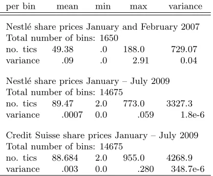
Table 1: Data characteristics
per bin mean min max variance
Nestl´e share prices January and February 2007 Total number of bins: 1650
no. tics 49.38 .0 188.0 729.07
variance .09 .0 2.91 0.04
Nestl´e share prices January – July 2009 Total number of bins: 14675
no. tics 89.47 2.0 773.0 3327.3 variance .0007 0.0 .059 1.8e-6
Credit Suisse share prices January – July 2009 Total number of bins: 14675
no. tics 88.684 2.0 955.0 4268.9 variance .003 0.0 .280 348.7e-6
Sources: Swiss stock exchange, own calculations.
1.3 million (Nestl´e and Credit Suisse each, 2009 sample) observations which are aggregated
into 1650 (Nestl´e, 2007 sample) and 14675 (Nestl´e and Credit Suisse each, 2009 sample) ten
and five minutes bins respectively. Table 1 on page 19 summarizes the data characteristics,
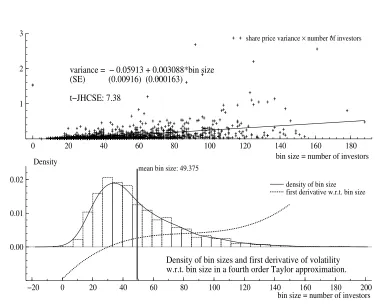
while figure 1 provides a plot of the 2007 Nestl´e data. In the top panel we see a cross
plot of the data while the bottom panel presents a non-parametric density estimate of the
number of observations, that is the sizes of the bin. These two plots already do suggest
that the variance tends to increase with the number of observed trades. Turning to formal
methods this impression is corroborated.
3.3 Empirical evidence across time, ...
Denoting the empirical price variance estimate ˆσ2t by ζt the following regressions analysis
sheds light on the relationship between variance and number of tics. Because the functional
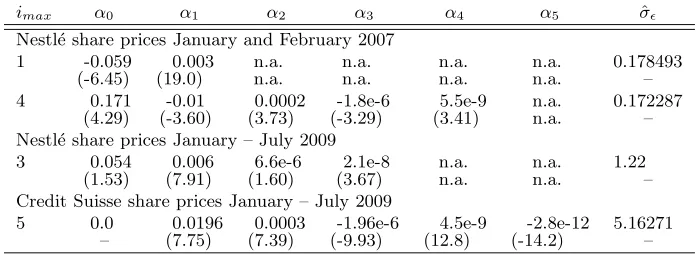
Table 2: Estimation results: Coefficient estimates and residual standard deviation
imax α0 α1 α2 α3 α4 α5 σˆǫ
Nestl´e share prices January and February 2007
1 -0.059 0.003 n.a. n.a. n.a. n.a. 0.178493
(-6.45) (19.0) n.a. n.a. n.a. n.a. –
4 0.171 -0.01 0.0002 -1.8e-6 5.5e-9 n.a. 0.172287
(4.29) (-3.60) (3.73) (-3.29) (3.41) n.a. – Nestl´e share prices January – July 2009
3 0.054 0.006 6.6e-6 2.1e-8 n.a. n.a. 1.22
(1.53) (7.91) (1.60) (3.67) n.a. n.a. –
Credit Suisse share prices January – July 2009
5 0.0 0.0196 0.0003 -1.96e-6 4.5e-9 -2.8e-12 5.16271
– (7.75) (7.39) (-9.93) (12.8) (-14.2) –
Coefficient estimates and correspondingt-values in parentheses below.
the true functional relationship between ζt and Nt to begin with:
ζt = α0+α1Nt+α2Nt2+· · ·+αimaxN
imax
t +ǫt
(5)
ǫt ∼ i.i.d.(0, σ2)
Although the variables exhibit a time subscript the regressions are essentially cross section
regressions. There may be occasions on which there are periods of generally higher or
particular lowζtaround but under the null hypothesis (the standard approach) this should
not be related toNt.
Applying standard model reduction technologies such as general-to-specific F-testing
and selection criteria (Akaike, Final Prediction Error, Schwarz) I derive a suitable
repre-sentation of the data. In most cases the optimal order seems to be four. Next, the first
derivative with respect to the number of observations within each bin is calculated and
evaluated for the data range. The following table collects the optimally fitting models and
in one instance (Nestl´e share prices in 2007) also a model variant where a simple linear
Yet another, nonparametric estimation of the relationship between bin size and
vari-ance is reported in the appendix. All methods deliver the same results qualitatively.
In the case where a simple linear model is estimated a standard t-test can be used
for evaluating the validity of the subjective model. The null hypothesis maintains the
standard case while the alternative corresponds to the subjective asset pricing model.
H0:α1 = 0 vs. H1 :α1 >0.
(6)
0 20 40 60 80 100 120 140 160 180
1 2 3
variance = − 0.05913 + 0.003088*bin size (SE) (0.00916) (0.000163)
t−JHCSE: 7.38
bin size = number of investors
share price variance × number of investors
−20 0 20 40 60 80 100 120 140 160 180 200
0.00 0.01 0.02
Density
Density of bin sizes and first derivative of volatility w.r.t. bin size in a fourth order Taylor approximation.
mean bin size: 49.375
bin size = number of investors
[image:22.612.102.477.278.583.2]density of bin size first derivative w.r.t. bin size
The estimation results are reported in table 2. They point strongly to a positive
relationship between the number of trades and the variance of the price. This is in stark
contrast to the usual conviction that more trades would reveal more information about
the true price. Instead of increasing the precision with which we measure the price by
using more observations it does in fact decrease.
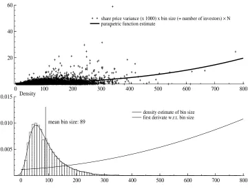
0 100 200 300 400 500 600 700 800
20 40 60
share price variance (x 1000) x bin size (= number of investors) × N parametric function estimate
0 100 200 300 400 500 600 700 800
0.005 0.010
0.015 Density
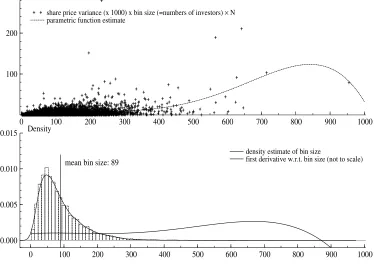
mean bin size: 89
[image:23.612.119.479.263.537.2]density estimate of bin size first derivate w.r.t. bin size
Because it is not easy to gauge the first derivative with respect to the number of
observations from the coefficient estimates, I provide plots of the derivatives. It turns
out that the first derivative is positive around the mean. This can be inferred from the
lower panel of figures 1 to 3 where the dotted (figure 1), or smooth solid line (figures 1,
2) marks the function of the first derivative.5 All in all there is little doubt that instead
of increasing the precision of our price measure the precision decreases when more trades
take place for any fixed information set.
0 100 200 300 400 500 600 700 800 900 1000
100 200
share price variance (x 1000) x bin size (=numbers of investors) × N parametric function estimate
0 100 200 300 400 500 600 700 800 900 1000
0.000 0.005 0.010
0.015 Density
mean bin size: 89
density estimate of bin size
[image:24.612.108.482.315.585.2]first derivative w.r.t. bin size (not to scale)
Figure 3: Credit Suisse 2009: Data plot and graphical estimation results
5
Interestingly, Lyons (2001), and Evans and Lyons (2002) observe similar effects when
they report the tremendous increase in the measure of fit of their exchange rate model.
The key variable they introduce is order flow data leading to an increase of up to 64%
in the measure of regression fit. Moreover, the variables which are in line with economic
theory are insignificant on all but one occasion. The result is similar to the present
since (cumulated) order flows are under fairly plausible assumptions proportionate to the
number of investors. Given the median model no wonder therefore, that Evans and Lyons
are able to explain a larger share of the variance.
The empirical results support the view that discouraging market participation by
ap-propriate means would reduce the price volatility. One such method could be the so-called
Tobin tax. As yet, it is too early to conclude that a Tobin tax would also be the optimal
tool, however.
The evidence presented here, could be challenged on grounds of endogeneity bias. If the
number of investors was dependent on the variance of the price process, then the regression
coefficients of equation (5) would not be reliable. Therefore, recent papers such as An´e
and Ureche-Rangau (2008) investigate the hypothesis that both number of trades (rather:
trading volume) and volatility are jointly determined by a latent number of information
arrivals. In our context this would imply that the five (ten) minutes time interval was
not short enough for keeping the information set constant. In the particular case of An´e
and Ureche-Rangau the data is daily price and volume of stocks which certainly justifies
modelling information arrivals. However, the general question whether or not trading
volume / number of traders is exogenous to the volatility remains.
In support of my regression approach I would like to point to the well-known lunchtime
exchange markets, or bond markets intra-day volatility assumes an U-shape (see e.g., Ito,
Lyons and Melvin, 1998; Hartmann, Manna and Manzanares, 2001, and the references
therein). Thus, following an exogenously determined decline in the number of investors
(traders) the volatility decreases justifying the assumption of weak exogeneity of numbers
of investors. The same U-shape pattern can be found in my data. For the sake of brevity
I do not report the details. They are available on request, however.
In sum, the empirical evidence is more in favour of the model presented in section 2
than in line with the traditional approach.
3.4 ..., space and markets
The previous sections provide evidence for abandoning the standard macro finance
ap-proach in favour of an alternative model that maintains individual rational behaviour
while emphasising the role of subjective rationality on the macro level.
However, there are at least two possibilities to match the data evidence with the
traditional view. One possibility is offered by infinite variance L´evy processes as price
generating processes. These processes also feature a higher variance the more data we
observe holding the information set constant. As regards the discrimination between the
subjective model and L´evy processes there is little one can do except from experiments.
Therefore, objective L´evy processes and the subjective asset pricing model probably
gen-erate data with very similar basic characteristics.
The second explanation could be that the five / ten minutes time interval is not short
enough for actually keeping the information set constant. If so, the increase in the variance
as more observations enter the intervall might simply be a reflection of a variation in the
Is this argument sufficient word of comfort for returning to the standard approach?
In my opinion it is not. The reason is very simple. While shares like Nestl´e’s are traded
every other second many of those assets which can be considered alternative investments
and hence conditioning variables in portfolio models, for example, may be traded far less
frequently. As an example consider the Swiss bond market. A safe alternative to the Swiss
shares would be Swiss government bonds. It can happen that those bonds are not traded
at all within hours. Therefore, the assumption made before finds support that within the
five / ten minutes time interval the information set remains constant.
Turning the argument around we would need to carefully synchronise the data of
inter-est and the information set, before we take up the standard approach again. Therefore, an
inevitable test of macro finance model would have to look at the high frequency data and
make sure that during those time spells where the conditioning variables do not change
the corresponding number of investors do not have explanatory power for the variance of
the dependent variable. So far, the standard procedure would be to synchronise
observa-tion data by using “suitable” time aggregates such as days, weeks, months, or quarters.
I do hazard the guess that the synchronisation exercise, however laborious, would always
produce the same result namely nonstationarity with respect to the number of trades.
Luckily, high quality data which permits such synchronisation exercise is becoming
more readily available. Very recently Akram, Rime and Sarno (2008) have investigated
arbitrage on foreign exchange markets, for example. Their high frequency data set consists
of matched spot, forward (forward swap) and deposit interest rate data for the currency
pairs British Pound / US Dollar, Euro / US Dollar, Japanese Yen / US Dollar. This data
will be used in the follwoing to corroborate the previous findings.
Pound but less so for the Euro and the Yen as Reuters is not the main trading platform in
these latter two cases. Moreover, the Japanese Yen is most heavily traded when Reuters
does not collect the data. Therefore, we will only look at the British Pound and the Euro
pairs.
Even though Akram et al. (2008) collect observations at the highest possible frequency
available to them there are occasions on which quotes for the swap, the spot, and the
interest rates do not occur simultaneously. Therefore, the variables with the lowest trading
activity set the limits. The most important effect on the data sample is a difference in the
number of observations despite an exact match of the sample period.
Of course, in order to test the model we need to track the market activity as closely
as possible. Whenever there are quotes for, say, the spot rate while there are no changes
in the interest rate we lose information. That’s why we again restrict our analysis to the
largest information sets.
The variable of interest is the arbitrage opportunity defined by the covered interest
parity condition given below
f xt=f xet
it
i∗
t
+et.
(7)
Equation (7) has it that the spot exchange rate (denoted f xt) must equal the forward
rate (f xet) up to deposit interest rate (it) on domestic assets discounted by the foreign
interest rate (i∗t) of the same maturities as the forward contract. As regards the actual
data bid and ask prices are available. Using ask and bid qoutes provides a much more
reliable picture of true arbitrage opportunities. Consequently, for each currency pair we
obtain two deviation measures.
A nonzeroetindicates arbitrage opportunities. Akram et al.’s (2008) analysis focusses
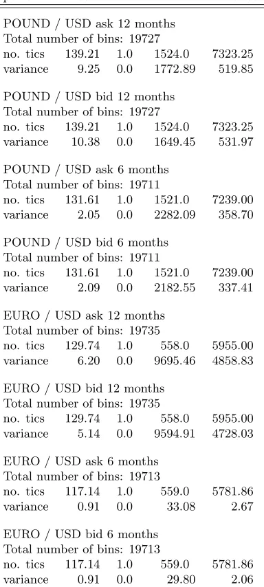
Table 3: CIP deviation data characteristics Feb – Sep 2004
per bin mean min max variance
POUND / USD ask 12 months Total number of bins: 19727
no. tics 139.21 1.0 1524.0 7323.25 variance 9.25 0.0 1772.89 519.85
POUND / USD bid 12 months Total number of bins: 19727
no. tics 139.21 1.0 1524.0 7323.25 variance 10.38 0.0 1649.45 531.97
POUND / USD ask 6 months Total number of bins: 19711
no. tics 131.61 1.0 1521.0 7239.00 variance 2.05 0.0 2282.09 358.70
POUND / USD bid 6 months Total number of bins: 19711
no. tics 131.61 1.0 1521.0 7239.00 variance 2.09 0.0 2182.55 337.41
EURO / USD ask 12 months Total number of bins: 19735
no. tics 129.74 1.0 558.0 5955.00 variance 6.20 0.0 9695.46 4858.83
EURO / USD bid 12 months Total number of bins: 19735
no. tics 129.74 1.0 558.0 5955.00 variance 5.14 0.0 9594.91 4728.03
EURO / USD ask 6 months Total number of bins: 19713
no. tics 117.14 1.0 559.0 5781.86 variance 0.91 0.0 33.08 2.67
EURO / USD bid 6 months Total number of bins: 19713
no. tics 117.14 1.0 559.0 5781.86 variance 0.91 0.0 29.80 2.06
but these are all very short lived. For the sake of brevity I do not describe the data in detail.
All those details are reported in Akram et al. (2008), the data has been downloaded from
Dagfinn Rime’s website. Rime also kindly provided advise in handling and interpretating
the data.
In what follows we will look at derived values foret for the two currency pairs Pound
/ US Dollar, and Euro / US Dollar. For each of these two pairs et is calculated for bid
and ask spot rates respectively. I investigate forward contracts for twelve and six months
because these are the most liquid markets and we therefore most likely obtain a fair picture
of the whole market. Taken together, eight data sets are available for analysis.
The observation period is February 13 to September 30, 2004, weekdays between 07:00
and 18:00 GMT which provides up to 2.7 million observations per currency pair and quote
(bid or ask). This data is again bundled into five minutes bins.
After going through the same steps of analysis as before it turns out that the standard
approach can again be rejected in basically all cases. The first derivative of the function
describing the relationship between bin size and variance is positive around mean / median,
and relying on nonparametric analysis, there is convincing evidence for this derivative to
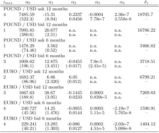
Table 4: Estimating CIP deviation variance: Coefficient estimates and residual standard
deviation
imax α0 α1 α2 α3 α4 ˆσǫ
POUND / USD ask 12 months
4 7485.59 -15.31 0.2237 -0.0004 2.36e-7 18705.7 (522.3) (8.94) 0.0456 7.78e-7 3.558e-8 – POUND / USD bid 12 months
1 7095.85 20.677 n.a. n.a. n.a. 16786.22
(380.6) (2.51) n.a. n.a. n.a. –
POUND / USD ask 6 months
1 1478.29 3.562 n.a. n.a. n.a. 3466.82
(74.46) (0.52) n.a. n.a. n.a. –
POUND / USD bid 6 months
3 1008.62 12.875 -0.0455 7.0e-5 n.a. 3718.51
(196.1) (3.451) (-0.017) (2.41e-5) n.a. – EURO / USD ask 12 months
2 1682.37 6.86 6.05 n.a. n.a. 6799.21
(86.96) (2.320) (0.012) n.a. n.a. –
EURO / USD bid 12 months
3 1667.63 38.67 -0.1445 0.0003 n.a. 7269.83
(188.8) (3.95) 0.0233 0.839e-5 n.a. –
EURO / USD ask 6 months
4 240.727 14.25 -0.0955 0.0003 -2.19e-7 1590.91 (45.56) (1.476) 0.0144 5.11e-5 5.765e-8 – EURO / USD bid 6 months
4 229.241 13.285 -0.086 0.0002 -2.03e-7 1404.12 (40.21) (1.303) 0.0127 4.51e-5 5.088e-8 –
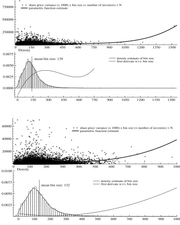
0 150 300 450 600 750 900 1050 1200 1350 1500 250000
500000
750000 share price variance (x 1000) x bin size (= number of investors) × N parametric function estimate
0 150 300 450 600 750 900 1050 1200 1350 1500
0.0000 0.0025 0.0050 0.0075
Density
mean bin size: 139 density estimate of bin size first derivate w.r.t. bin size
0 100 200 300 400 500 600 700 800 900 1000
20000 40000
60000 share price variance (x 1000) x bin size (= number of investors) × N
parametric function estimate
0 100 200 300 400 500 600 700 800 900 1000
0.0025 0.0050 0.0075
0.0100 Density
mean bin size: 132
[image:32.612.115.479.153.608.2]density estimate of bin size first derivate w.r.t. bin size
Figure 4: UIP one year ask (top panel) and six months bid (bottom panel) British Pound
0 50 100 150 200 250 300 350 400 450 500 550 600 50000
100000 150000
share price variance (x 1000) x bin size (= number of investors) × N parametric function estimate
0 50 100 150 200 250 300 350 400 450 500 550 600
0.0025 0.0050 0.0075
0.0100 Density
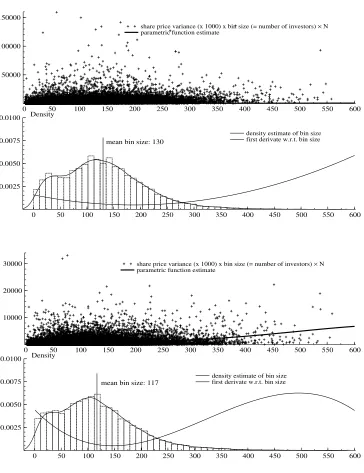
mean bin size: 130
density estimate of bin size first derivate w.r.t. bin size
0 50 100 150 200 250 300 350 400 450 500 550 600
10000 20000
30000 share price variance (x 1000) x bin size (= number of investors) × N parametric function estimate
0 50 100 150 200 250 300 350 400 450 500 550 600
0.0025 0.0050 0.0075
0.0100 Density
mean bin size: 117
[image:33.612.118.482.140.613.2]density estimate of bin size first derivate w.r.t. bin size
Figure 5: UIP one year bid (top panel) and six months ask (bottom panel) Euro / US
3.5 Reconciling evidence from experiments
The empirical investigation showed that the data has properties which one would expect
if investors behaved according to the median model. However, the median model poses
the absence of an objective price process and this absence is impossible to prove since
the non-existing can not be proven to not exist. Therefore, the empirical evidence can
be interpreted as an as if behaviour. Investors behave as if there was no objective price
process. This interpretation also holds the key for reconciling experimental evidence of
investors’ behaviour.
The first stylised fact is the so-called irrational behaviour in artificial asset
mar-kets (see inter alia Smith et al., 1988; Cipriani and Guarino, 2005). It has likewise be
demonstrated that experienced traders can push the market price towards its
funda-mental value and hence eradicate irrational prices (see e.g. Dufwenberg, Lindqvist and
Moore, 2005; Drehmann, Oechssler and Roider, 2005; Hussam, Porter and Smith, 2008,
to name but a few). Notably, all these experiments use a design in which an (implicit)
objective price process is induced. For example, the traded asset may yield a return with
a given probability each period. Therefore, irrationality in such a situation might be used
as an argument against the median model. I prefer a different interpretation, however.
The participants in these experiment behave exactly as they would have done in the real
world: they trade as if there was no objective price process. By contrast, expert traders are
able to discover the induced pricing rule and hence tend to behave rationally. Therefore,
these experiments do not lend support to the standard approach. The decisive question is
how do experts trade in the absence of an objective price process? Thus, the need for an
accordingly set up experiment remains and economists might have a closer look at optimal
Therefore, in the light of more realistic properties of the theoretical model I consider
the conclusion of rational “irrationality” of asset markets the more plausible one.
Alternatively, one may regard each tic as a piece of information itself. In the logic of
my argument each investor would represent an indispensable piece of information. The
standard REH approach would thus have to include each investor in the information
set.6 Then, the standard approach and my model would generate data which would be
observationally equivalent.
4
Summary and conclusions
The observation of a price for an asset is no proof for this price to follow a discoverable,
objective stochastic process. In this paper I discuss a model for the determination of asset
prices which emphasises the role of subjective probability distribution functions for the
price process. It generalises models which are based on concepts of objective probability
functions. Next to being less restrictive the new model can be regarded as simpler. A
test has been suggested with the traditional view as the null hypothesis and the new
approach in the alternative. Empirical investigations covering many data sets across time,
space, and markets found strong support for rejecting the Null. Allowing for subjectivity
in financial markets helps understanding major pricing puzzles. It also lends tentative
support to the Tobin tax for reducing asset price volatility. The new model implies an
alternative research agenda which focuses on optimal decision making under fundamental
uncertainty.
6
References
Akram, Q. F., Rime, D. and Sarno, L. (2008). Arbitrage in the foreign exchange market:
Turning on the microscope, Journal of International Economics76(2): 237–253.
An´e, T. and Ureche-Rangau, L. (2008). Does trading volume really explain stock
re-turns volatility?,Journal of International Financial Markets, Institutions and Money
18(3): 216–235.
Bacchetta, P. and van Wincoop, E. (2005). Rational Inattention: Solution to the Forward
Discount Puzzle, Research Paper 156, International Center for Financial Asset and
Engineering.
Barndorff-Nielsen, O. E. and Shepard, N. (2002). Econometric Analysis of Realised
Volatil-ity and its Use in Estimating Stochastic VolatilVolatil-ity Modells, Journal of the Royal
Statistical Society, Series B64: 253 – 280.
Branch, W. A. (2004). The theory of rationally heterogenous expectations: Evidence from
survey data,The Economic Journal 114: 592 – 621.
Cheung, Y.-W., Chinn, M. D. and Pascual, A. G. (2005). Empirical exchange rate models
of the nineties: Are any fit to survive?,Journal of International Money and Finance
19: 1150 – 1175.
Cipriani, M. and Guarino, A. (2005). Herd Behavior in a Laboratory Financial Market,
American Economic Review95(5): 1427–1443.
Conlisk, J. (1996). Why bounded rationality?, Journal of Economic Literature34(2): 669
Downs, A. (1957). An Economic Theory of Democracy, Harper and Row, New York.
Drehmann, M., Oechssler, J. and Roider, A. (2005). Herding and Contrarian
Behav-ior in Financial Markets: An Internet Experiment, American Economic Review
95(5): 1403–1426.
Dufwenberg, M., Lindqvist, T. and Moore, E. (2005). Bubbles and experience: An
exper-iment,American Economic Review95(5): 1731–1737.
Evans, M. D. D. and Lyons, R. K. (2002). Order flow and exchange rate dynamics,Journal
of Political Economy 110(1): 170 – 180.
Friedman, M. (1953). The Case of Flexible Exchange Rated,inM. Friedman (ed.), Essays
in Positive Economics, University of Chicago Press, Chicago, pp. 157–203.
Grauwe, P. D. and Kaltwasser, P. R. (2007). Modeling optimism and pessimism in the
foreign exchange market,CESifo Working Paper Series 1962, CESifo GmbH.
Hartmann, P., Manna, M. and Manzanares, A. (2001). The microstructure of the euro
money market,Journal of International Money and Finance20(6): 895–948.
Hussam, R. N., Porter, D. and Smith, V. L. (2008). Thar She Blows: Can Bubbles Be
Rekindled with Experienced Subjects?,American Economic Review98(3): 924–937.
Ito, T., Lyons, R. K. and Melvin, M. T. (1998). Is There Private Information in the FX
Market? The Tokyo Experiment,Journal of Finance53(3): 1111–1130.
Lyons, R. K. (2001). Foreign exchange: macro puzzles, micro tools,Pacific Basin Working
Nerlove, M. (1983). Expectations, Plans, and Realizations in Theory and Practice,
Econo-metrica 51(2): 1251 – 1280.
Obstfeld, M. and Rogoff, K. (2000). The six major puzzles in international
macroeco-nomics: Is there a common cause?, Working Paper 7777, National Bureau of
Eco-nomic Research.
Pesaran, H. M. (1987). The Limits to Rational Expectations, Basil Blackwell, Oxford.
Salvatore, D. (2005). The euro-dollar exchange rate defies prediction, Journal of Policy
Modelling27(2): 455 – 464.
Shleifer, A. and Summers, L. H. (1990). The noise trader approach to finance, Journal of
Economic Perspectives 4(2): 19 – 33.
Sims, C. (2005). Rational inattention: A research agenda, Discussion Paper, Series 1:
Economic Studies 34, Deutsche Bundesbank.
Smith, V. L., Suchanek, G. L. and Williams, A. W. (1988). Bubbles, crashes, and
endoge-nous expectations in experimental spot asset markets,Econometrica56(5): 1119–51.
Taylor, M. P. (1995). The economics of exchange rates, Journal of Economic Literature
33(1): 13 – 47.
Tirole, J. (2002). Rational irrationality: Some economics of self-management, European
Economic Review46(4 – 5): 633 – 655.
Verma, R. and Verma, P. (2007). Noise trading and stock market volatility, Journal of
Wang, P. and Jones, T. (2003). The Impossibility of Meaningful Efficient Market
Param-eters in Testing for the Spot–Foreward Relationship in Foreign Exchange Markets,
Economics Letters81: 81 – 87.
A
Nonparametric estimation of the bin size – variance
re-lationship
Equation (5) defines a parametric function of the relation between bin size (the
approxima-tion of number of traders) and the variance of the asset price within those five / ten minute
time bins. The according results lend support to the hypothesis of a positive association
between the number of trades and the variance of the asset price. Nevertheless, one may
wonder to what extent these results depend on the specific parametric functional forms
used. Therefore, I report the outcome of a nonparametric, local quadratic estimation of
the relation between bin size and variance.
The estimation is based on the software XploRe which is specifically designed for
analysing financial market data by means of non- and semi-parametric functions.7 In
particular, I make use of the procedure “lplocband” of the “smoother” library applying
the Epanechnikov kernel. The kernel bandwidth is chosen manually because the automatic
procedures always selected the lowest possible bandwidth within the pre-defined range.
These lower bands were close to the minimum distance between any two explanatory
variable data points. The results do not change qualitatively, however, within a large
range of bandwidths.
7
Figure 6: Random walk: Nonparametric estimation of bin size – variance relation and
Before turning to the empirical evidence let me reconcile the results which could be
expected under the null hypothesis, the standard approach. Figure 6 plots observations
that are generated by simulating 14675 random walks of length 955. In the next step,
between 2 and 955 data points of these random walks are selected randomly from each
of the 14675 data sets. These observations mimic the five minutes bins. Accordingly,
the variance of these bins is estimated and set in relation to the number of artificial
observations entering the bin. This simulation procedure thus draws on the actual Credit
Suisse data and clearly demonstrates that even under the random walk hypothesis for
price data the relationship between bin size and variance should be completely stochastic;
the first derivative estimate frequently crosses the zero line, and the 95 percent confidence
bands safely enclose zero.
By contrast, the empirical relationships do look pretty different. For example figure 7
shows that the estimated first derivative is significantly larger than zero around the mean
bin size in the case of the 2007 Nestl´e data. Very similar pictures emerge for the other
data sets.
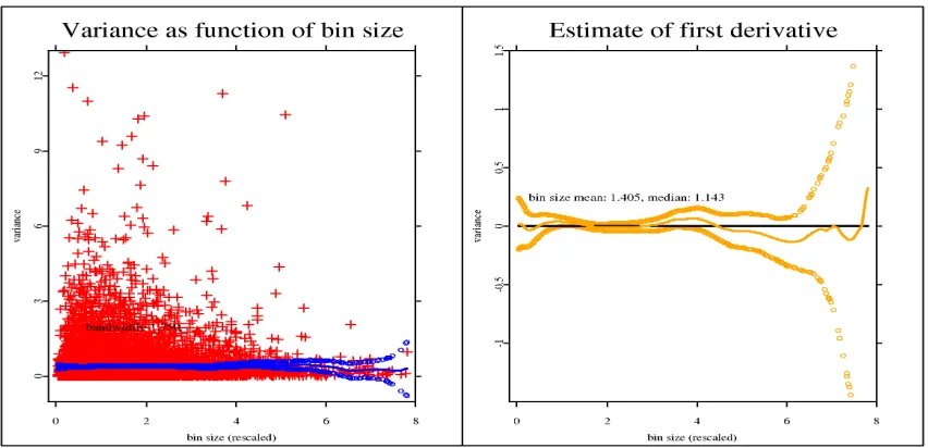
In some instances (see figure 11 on p. 46), there are also hints for another phenomenon.
In these instances the relationship between variance and bin size seems to be negative.
This situation occurs when trading volume is low (small bin sizes) and gives rise to the
possibility of dependent observations. For example, when trading activity is low, several
consecutive trades may be exercised by the same trader(s).
In order to render the estimation feasible, i.e. avoiding numerical problems, the
inde-pendent variable was divided by twice the maximum value of the bin size. If that was not
sufficient to overcome numerical problems both variables were normalised by their
Variance as function of bin size
0 0.1 0.2 0.3 0.4
bin size (rescaled)
0
0.5
1
1.5
2
2.5
variance
bandwidth: 0.225
Estimate of first derivative
0 0.1 0.2 0.3 0.4
bin size (rescaled)
-10
0
10
20
variance
[image:42.612.103.526.151.367.2]bin size mean: 0.119, median: 0.102
Figure 7: Nestl´e tic data 2007: Nonparametric estimation of bin size – variance relation
and its first derivative
Figure 8: Nestl´e tic data 2009 (top panel) and Credit Suisse tic data 2009 (bottom panel):
Pretty much in line with the parametric estimation the variance increases with the bin
size. The panel on the left shows an upward trend in the variance for growing bin sizes and
the panel to the right confirms that the first derivative of the relationship is significantly
larger than zero around the mean bin size and for sizes larger than the mean. Therefore,
the hypothesis derived from the median model receives support once more.
B
Evidence from foreign exchange markets
The following graphs depict the results for the data compiled by Akram et al. (2008).
Here, the data is always standardized such that the empirical variance of dependent and
independent variable is one. As before, this linear transformation cannot affect their
Variance as function of bin size
0 1 2 3 4 5 6 7 8
bin size (rescaled)
0 0 0 0 0 variance (rescaled)*E7 bandwidth: 1.750
Estimate of first derivative
0 1 2 3 4 5 6 7 8
bin size (rescaled)
0
0
0
0
variance (rescaled)*E7 bin size mean: 1.630, median: 1.474
Variance as function of bin size
0 1 2 3 4 5 6 7 8
bin size (rescaled)
0 0 0 0 0 0 variance (rescaled)*E7 bandwidth: 1.750
Estimate of first derivative
0 1 2 3 4 5 6 7 8
bin size (rescaled)
0
0
0
0
variance (rescaled)*E7
[image:45.612.91.541.139.602.2]bin size mean: 1.630, median: 1.474
Figure 9: Pound one year ask (top panel) and bid (bottom panel): Nonparametric
Variance as function of bin size
0 1 2 3 4 5 6 7 bin size (rescaled)
0
0
0
0
variance (rescaled)*E7
bandwidth: 1.750
Estimate of first derivative
0 0.5 1 1.5 2 2.5 3 3.5 4 4.5 5 5.5 6 6.5 7 bin size (rescaled)
0
variance (rescaled)*E7
bin size mean: 1.550, median: 1.365
Variance as function of bin size
0 1 2 3 4 5 6 7 bin size (rescaled)
0
0
0
0
variance (rescaled)*E7
bandwidth: 1.750
Estimate of first derivative
0 0.5 1 1.5 2 2.5 3 3.5 4 4.5 5 5.5 6 6.5 7 bin size (rescaled)
0
[image:46.612.91.540.142.603.2]variance (rescaled)*E7 bin size mean: 1.550, median: 1.365
Figure 10: Pound 6 months ask (top panel) and bid (bottom panel): Nonparametric
Variance as function of bin size
0 1 2 3 4 5 6 7
bin size (rescaled)
1 2 3 4 5 6 variance (rescaled) bandwidth: 1.750
Estimate of first derivative
0 0.5 1 1.5 2 2.5 3 3.5 4 4.5 5 5.5 6 6.5 7
bin size (rescaled)
0
0.5
1
1.5
variance (rescaled)
bin size mean: 1.548, median: 1.423
Variance as function of bin size
0 1 2 3 4 5 6 7
bin size (rescaled)
1 2 3 4 5 6 variance (rescaled) bandwidth: 1.750
Estimate of first derivative
0 1 2 3 4 5 6 7
bin size (rescaled)
0
0.5
1
1.5
variance (rescaled)
[image:47.612.110.489.158.568.2]bin size mean: 1.548, median: 1.423
Figure 11: Euro 6 months ask (top panel) and bid (bottom panel): Nonparametric
Variance as function of bin size
0 1 2 3 4 5 6 7
bin size (rescaled)
0
0.5
1
1.5
2
variance (rescaled)
bandwidth: 1.750
Estimate of first derivative
0 0.5 1 1.5 2 2.5 3 3.5 4 4.5 5 5.5 6 6.5 7
bin size (rescaled)
0
0.25
0.5
variance (rescaled)
bin size mean: 1.690, median: 1.598
Variance as function of bin size
0 1 2 3 4 5 6 7
bin size (rescaled)
0
0.5
1
1.5
variance (rescaled)
bandwidth: 1.750
Estimate of first derivative
0 0.5 1 1.5 2 2.5 3 3.5 4 4.5 5 5.5 6 6.5 7
bin size (rescaled)
0
0.5
variance (rescaled)
[image:48.612.109.493.157.568.2]bin size mean: 1.690, median: 1.598
Figure 12: Euro 12 months ask (top panel) and bid (bottom panel): Nonparametric